9.9. Visualization#

The IoT plotting layer lives in pycsamt.iot.plot and is re-exported from pycsamt.iot. These figures are operational acquisition plots: they show telemetry health, edge decisions, power budget, and clock synchronisation before the data are converted into impedance products or inversion inputs. Every function covered on this page has already appeared once elsewhere in this guide — plot_field_dashboard() in Basic Session and Telemetry Transports, plot_edge_qc_summary() in Generic Edge QC — but always attached to the topic that page was teaching. Here they are the subject: what each panel actually plots, where its numbers come from, and which function to reach for first.

The plotting functions accept high-level objects such as FieldSession, telemetry packets, energy estimates, synchronisation status objects, or serialised mappings. Each returned Matplotlib figure also carries the normalised plot data used to draw the panels in a fig.pycsamt_iot_* attribute. That makes report generation auditable: the image and the plotted rows stay together, so a reviewer can reconstruct exactly what a bar or point represents without re-deriving it from the raw packets.

9.9.1. Building A Visualisation Session#

This example uses synthetic data built deterministically from a fixed seed. It creates three stations on profile L18: one healthy, one with poor finite coverage on one channel, and one with a spike on another. Each station gets a QC packet (run through the same EdgeProcessor introduced in Generic Edge QC), a health packet, a power packet, and a sync packet, so every one of the four plotting functions below has real data to draw. With \(N_s=3\) stations and four packets each, the total is \(4N_s=12\).

>>> import numpy as np
>>> from pycsamt.iot import (
...     DeviceConfig, EdgeProcessingConfig, EdgeProcessor, EnergyConfig,
...     FieldSession, MonitoringConfig, PacketKind, StationConfig,
...     TelemetryPacket, estimate_energy_budget,
... )
>>> survey_id = "WILLY-L18-VISUAL"
>>> station_ids = ["L18-001", "L18-002", "L18-003"]
>>> positions_m = [0.0, 50.0, 100.0]
>>> coords = [(7.501, -5.201), (7.502, -5.198), (7.503, -5.195)]
>>> devices = [
...     DeviceConfig(
...         f"l18-node-{i + 1:02d}", station=sid,
...         channels=["ex", "ey", "hx", "hy"], sample_rate_hz=256.0,
...     )
...     for i, sid in enumerate(station_ids)
... ]
>>> stations = [
...     StationConfig(
...         sid, profile="L18", position_m=pos, lat=lat, lon=lon,
...         channels=["ex", "ey", "hx", "hy"],
...     )
...     for sid, pos, (lat, lon) in zip(station_ids, positions_m, coords)
... ]
>>> session = FieldSession(
...     survey_id, devices=devices, stations=stations,
...     monitoring_config=MonitoringConfig(
...         method="amt", expected_interval_s=6.0, max_gap_s=18.0,
...         min_edge_acceptance_rate=0.70, min_battery_v=11.2,
...         required_channels=["ex", "ey", "hx", "hy"],
...     ),
... )
>>> processor = EdgeProcessor(
...     EdgeProcessingConfig(
...         decimation=1, finite_threshold=0.85, warn_finite_threshold=0.95,
...         channel_names=["ex", "ey", "hx", "hy"], spike_threshold=4.0,
...         max_spike_fraction=0.12,
...     )
... )
>>> rng = np.random.default_rng(42)
>>> battery_v = [12.55, 11.84, 10.92]
>>> temperature_c = [30.1, 31.4, 33.2]
>>> battery_wh = [180.0, 120.0, 70.0]
>>> active_power_w = [1.2, 1.6, 2.1]
>>> duty_cycle = [0.25, 0.35, 0.55]
>>> solar_wh_per_day = [8.0, 3.0, 0.0]
>>> sync_specs = [
...     {"offset_ms": 0.32, "drift_ppm": 1.4, "jitter_ms": 0.16,
...      "gps_lock": True, "n_reference_points": 120, "quality": "excellent"},
...     {"offset_ms": 1.84, "drift_ppm": 11.2, "jitter_ms": 0.72,
...      "gps_lock": True, "n_reference_points": 118, "quality": "fair"},
...     {"offset_ms": 7.62, "drift_ppm": 69.5, "jitter_ms": 2.15,
...      "gps_lock": False, "n_reference_points": 61, "quality": "poor"},
... ]
>>> for idx, device in enumerate(devices):
...     data = rng.normal(size=(256, 4))
...     if idx == 1:
...         data[20:230, 1] = np.nan
...     if idx == 2:
...         data[80:125, 0] = 15.0
...     edge = processor.process(data)
...     qc_packet = edge.to_packet(
...         device, timestamp=1_700_000_000.0 + idx * 6.0,
...         survey_id=survey_id, qos=1,
...     )
...     qc_packet.payload["station"] = device.station
...     qc_packet.payload["method"] = "amt"
...     _ = session.add_packet(qc_packet)
...     health = TelemetryPacket.from_device(
...         device, timestamp=1_700_000_002.0 + idx * 6.0,
...         survey_id=survey_id, kind=PacketKind.HEALTH,
...         payload={
...             "station": device.station, "battery_v": battery_v[idx],
...             "temperature_c": temperature_c[idx],
...         },
...     )
...     _ = session.add_packet(health)
...     power_config = EnergyConfig(
...         battery_wh=battery_wh[idx], active_power_w=active_power_w[idx],
...         sleep_power_w=0.18, duty_cycle=duty_cycle[idx],
...         solar_wh_per_day=solar_wh_per_day[idx], telemetry_power_w=2.0,
...         telemetry_seconds_per_day=600.0, edge_power_w=0.35,
...         edge_duty_cycle=0.20, min_runtime_days=5.0,
...         device_id=device.device_id,
...     )
...     power_packet = estimate_energy_budget(power_config).to_packet(
...         device, timestamp=1_700_000_004.0 + idx * 6.0, survey_id=survey_id,
...     )
...     power_packet.payload["station"] = device.station
...     _ = session.add_packet(power_packet)
...     sync_payload = dict(sync_specs[idx], station=device.station)
...     _ = session.add_packet(
...         TelemetryPacket.from_device(
...             device, timestamp=1_700_000_006.0 + idx * 6.0,
...             survey_id=survey_id, kind=PacketKind.SYNC, payload=sync_payload,
...         )
...     )
>>> print((session.survey_id, session.n_devices, session.n_stations, session.n_packets))
('WILLY-L18-VISUAL', 3, 3, 12)

9.9.2. The Field Dashboard#

plot_field_dashboard() is the at-a-glance field dashboard: station health, edge-QC acceptance, power or synchronisation state, and packet timing in four panels. Internally it starts from session.to_pipeline_input() and the packet stream, then joins the latest battery voltage, runtime, power state, clock offset, and sync quality onto each station row. A station is marked critical when its power state is critical, its sync quality is poor, or its acceptance rate is below 0.85; it is marked warning when the acceptance rate is below 0.95 or when power/sync is warning/fair. The acceptance panel displays \(A_i=n_{\mathrm{accepted},i}/n_{\mathrm{qc},i}\) for each station, and the timeline uses minutes since the first finite packet timestamp.

>>> from pycsamt.iot import plot_field_dashboard
>>> dashboard = plot_field_dashboard(
...     session, now=1_700_000_030.0, station_axis="profile",
...     title="IoT field dashboard: WILLY L18",
... )
>>> dashboard_data = dashboard.pycsamt_iot_dashboard
>>> print(f"dashboard_stations: {len(dashboard_data['stations'])}")
dashboard_stations: 3
>>> print(f"dashboard_packets: {len(dashboard_data['packets'])}")
dashboard_packets: 12
>>> print(f"monitoring_level: {dashboard_data['monitoring']['level']}")
monitoring_level: critical
>>> print(f"issues: {', '.join(dashboard_data['issues']) or '-'}")
issues: battery_below_threshold, edge_acceptance_rate_below_threshold, required_channels_missing

station_axis only changes one of the four panels: "profile" lays stations out by chainage, while "map" uses longitude/latitude — and since every station here carries real coordinates, both are worth seeing side by side rather than picking one arbitrarily. The script below rebuilds the session and saves the "profile" dashboard shown as the first figure further down:

The map variant changes nothing but that one keyword argument — same session, same thresholds, just station_axis="map" — and saves the second figure:

../../_images/user-guide-iot-visualization-01.png

../../_images/user-guide-iot-visualization-05.png

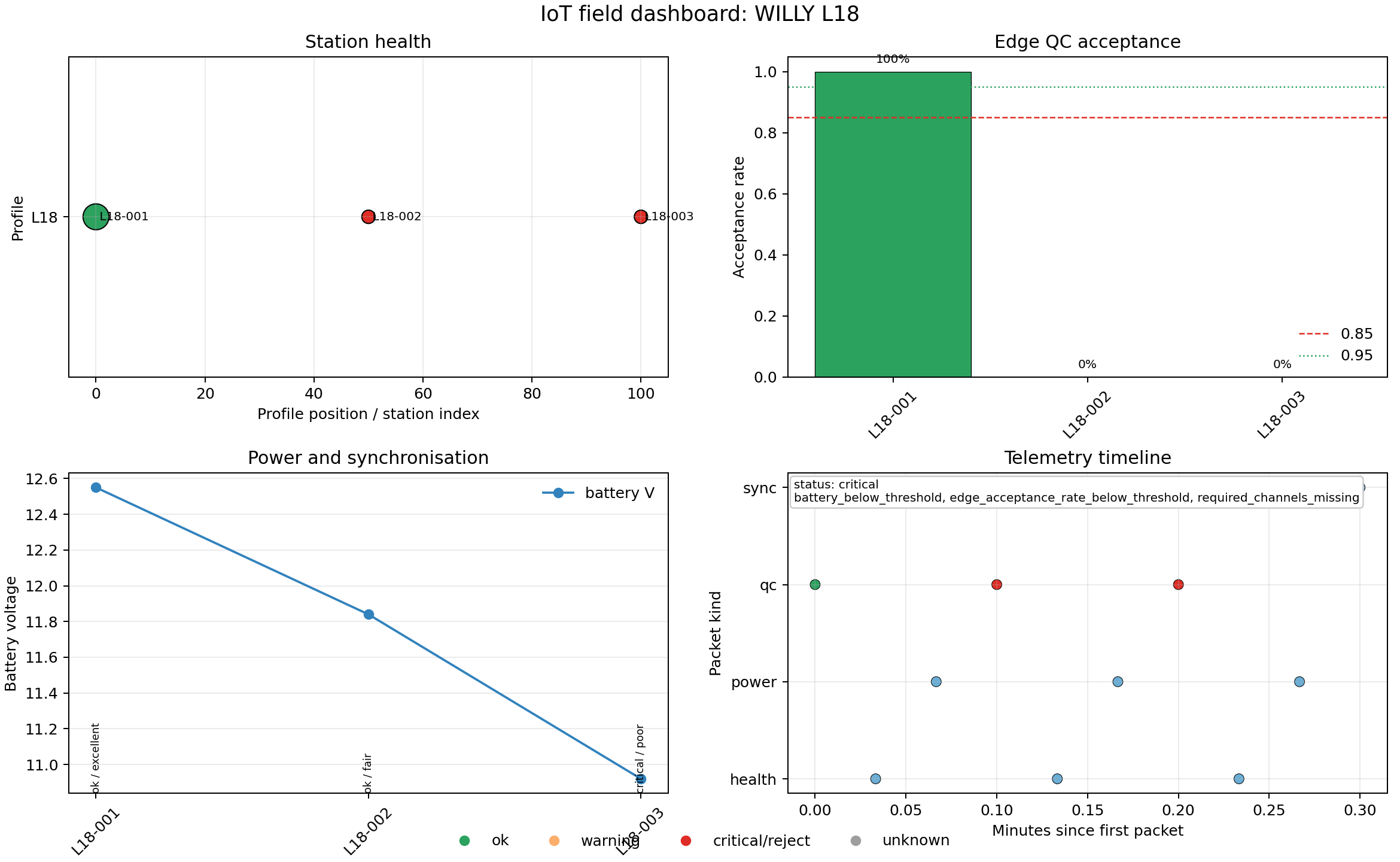
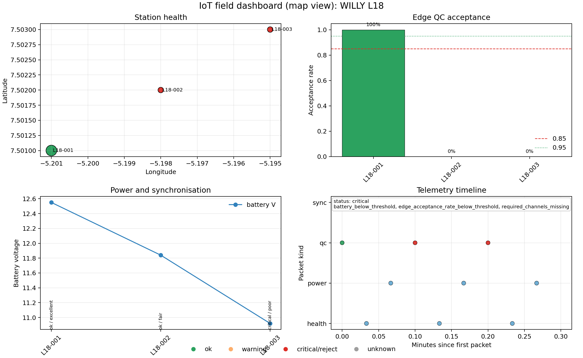
The station-health panel is the only thing that changes between the two: chainage 0/50/100 m becomes longitude/latitude, and L18-001 stays the one large green marker in both. The other three panels — acceptance, power/sync, timeline — read from the same station and packet rows regardless of axis choice, so they are pixel-identical between the two figures. Reach for "map" once a survey is no longer a single straight line and chainage stops being a meaningful x-axis; use "profile" for ordinary line work, which is the more common case and the default this guide otherwise uses.

9.9.3. Edge QC Detail#

Use plot_edge_qc_summary() when the dashboard indicates that edge quality is the problem — the same function Generic Edge QC introduced on synthetic windows, now reading straight from a session. It accepts a FieldSession, one or more QC telemetry packets, or raw EdgeProcessingResult objects, and normalises whichever it receives into one row per station/channel pair. From that row set it counts decisions, plots finite coverage against the configured warning/rejection thresholds, plots robust spike fraction, and tallies rejection or warning reasons — each window-level reason once per window, each channel-level reason once per channel, exactly as derived in Generic Edge QC.

>>> from pycsamt.iot import plot_edge_qc_summary
>>> qc_fig = plot_edge_qc_summary(session, title="Edge QC visual summary: WILLY L18")
>>> qc_rows = qc_fig.pycsamt_iot_edge_qc
>>> print(f"qc_rows: {len(qc_rows)}")
qc_rows: 12
>>> print(f"qc_decisions: {sorted({row['decision'] for row in qc_rows})}")
qc_decisions: ['accept', 'reject']
>>> print(f"qc_channels: {sorted({row['channel'] for row in qc_rows})}")
qc_channels: ['ex', 'ey', 'hx', 'hy']

../../_images/user-guide-iot-visualization-02.png

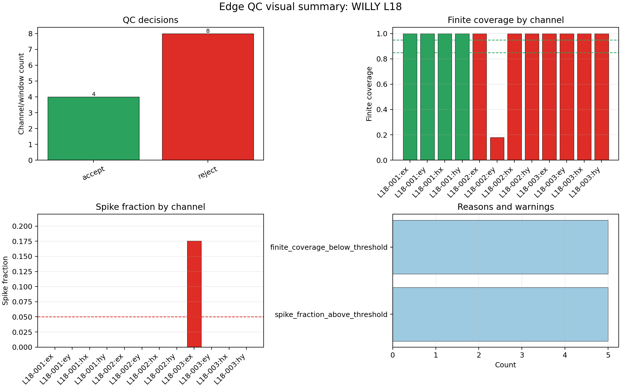
All four of L18-001’s channels are green and accepted; all eight channels across the other two stations are red and rejected, matching the dashboard’s stream-wide acceptance already shown above. The coverage panel isolates exactly where: L18-002:ey alone drops to about 0.18, the injected NaN block from the session-building step, while every other channel — including L18-002’s other three — sits at a clean 1.0. The spike panel is the mirror image, flagging only L18-003:ex, where the 15.0 outlier was injected. The reasons panel totals two occurrences of each failure kind, not four or eight: one window-level reason per rejected station plus one matching channel-level reason from the specific channel that triggered it, counted the way Generic Edge QC derived rather than repeated once per channel in the row set.

9.9.4. Power Budgets#

Use plot_power_budget() to compare daily load, harvest, runtime, and power states. The input can be a session containing power packets, a list of EnergyConfig objects, power telemetry packets, or energy estimates. The first panel compares daily load \(L_i\) with harvested energy \(H_i\); the runtime panel compares estimated runtime \(T_i=E_{\mathrm{usable},i}/\max(L_i-H_i,0)\) with no-harvest autonomy; the breakdown panel stacks base, telemetry, edge-processing, and auxiliary load components so the sum returns \(L_i\). The final panel counts power state values and lists the most common issues.

>>> from pycsamt.iot import plot_power_budget
>>> power_fig = plot_power_budget(session, title="Power budget visual summary: WILLY L18")
>>> power_rows = power_fig.pycsamt_iot_power_budget
>>> print(f"power_rows: {len(power_rows)}")
power_rows: 3
>>> print(f"power_states: {sorted({row['state'] for row in power_rows})}")
power_states: ['critical', 'ok']
>>> print(
...     "runtime_days: "
...     + ", ".join(
...         "inf" if np.isinf(row["runtime_days"]) else f"{row['runtime_days']:.2f}"
...         for row in power_rows
...     )
... )
runtime_days: 40.42, 7.86, 2.21

../../_images/user-guide-iot-visualization-03.png

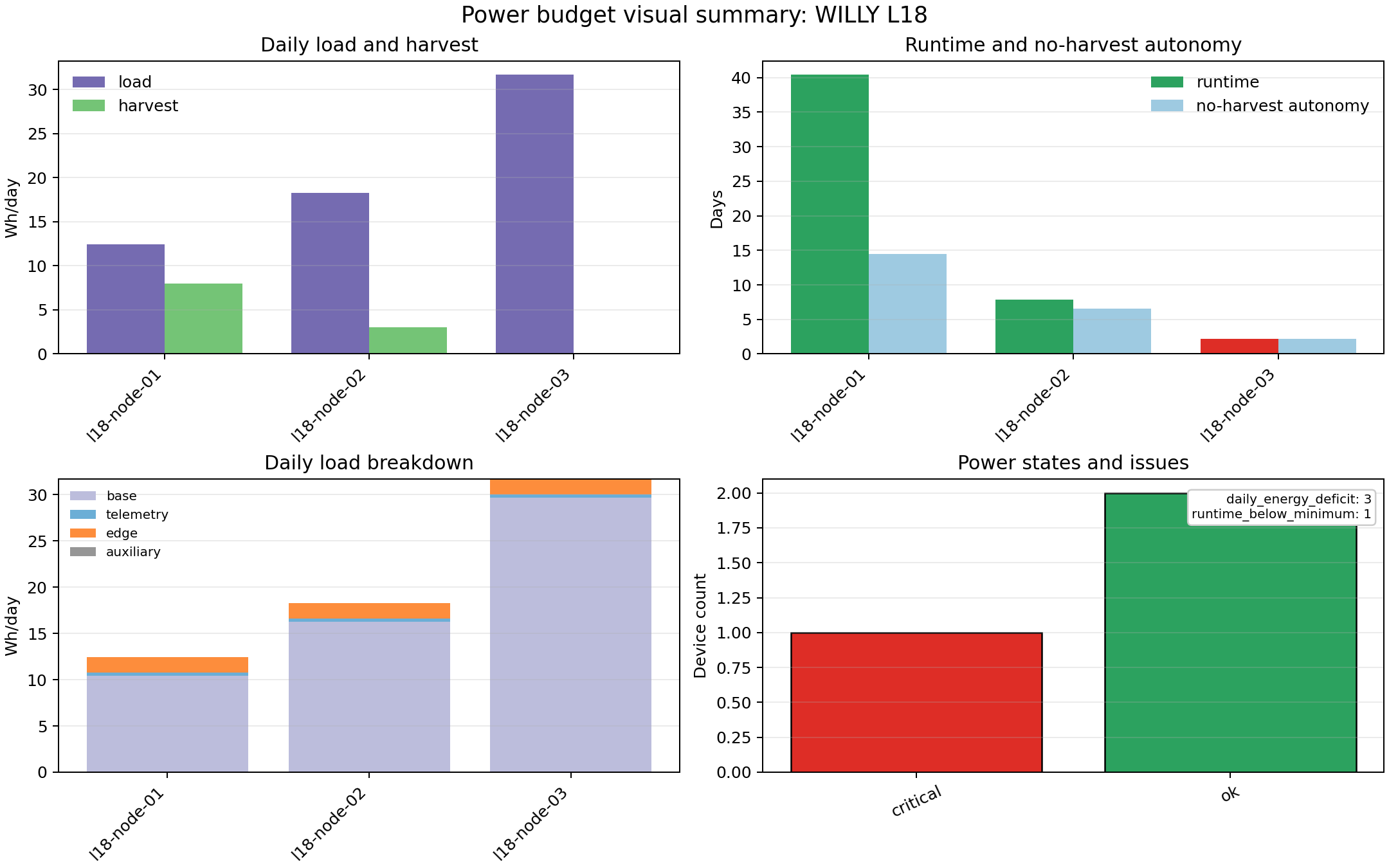
l18-node-03 is the node to worry about: its load/harvest panel shows a full purple load bar and no green harvest bar at all — zero solar input was deliberately configured for that node — and its runtime bar in the second panel barely clears the x-axis at 2.21 days, coloured red for critical while the other two stay green. The breakdown panel shows why the load itself is so much higher than the other two nodes: base load dominates every bar, but l18-node-03’s base load alone (about 29.7 Wh/day) is nearly triple l18-node-01’s (about 10.4 Wh/day), consistent with its higher configured active_power_w and duty cycle. The states panel’s issue list — daily_energy_deficit on three devices, runtime_below_minimum on one — makes explicit that a negative harvest margin and an unacceptably short runtime are two different thresholds, not the same check reported twice.

9.9.5. Clock Synchronisation#

Use plot_sync_quality() to inspect offset, drift, jitter, reference support, GPS lock, and quality grades. Threshold arguments draw reference lines but do not mutate the data. Each sync row carries the same quantities used by the clock-sync audit: clock offset \(o_i\), clock drift \(d_i\), timing jitter \(j_i\), GPS lock, and the number of reference points. The visual thresholds are overlays only: a tolerance line at \(|o|=o_{\max}\), a drift line at \(|d|=d_{\max}\), and a jitter line at \(j=j_{\max}\).

>>> from pycsamt.iot import plot_sync_quality
>>> sync_fig = plot_sync_quality(
...     session, title="Clock sync visual summary: WILLY L18",
...     tolerance_ms=1.0, max_drift_ppm=10.0, max_jitter_ms=1.0,
... )
>>> sync_rows = sync_fig.pycsamt_iot_sync_quality
>>> print(f"sync_rows: {len(sync_rows)}")
sync_rows: 3
>>> print(f"sync_quality: {sorted({row['quality'] for row in sync_rows})}")
sync_quality: ['excellent', 'fair', 'poor']
>>> print(f"gps_lock_values: {[row['gps_lock'] for row in sync_rows]}")
gps_lock_values: [True, True, False]

../../_images/user-guide-iot-visualization-04.png

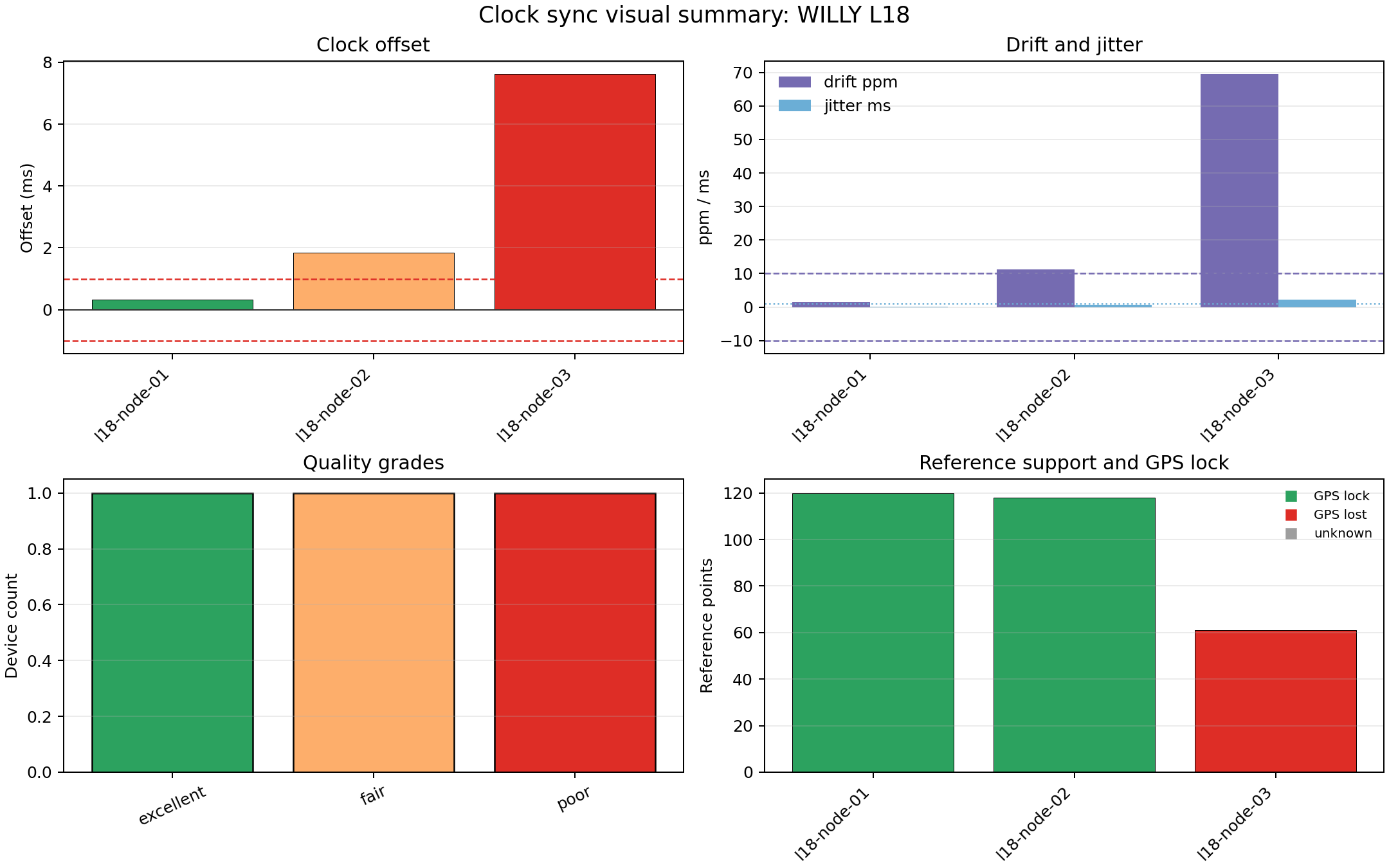
l18-node-03 again stands out, and for a related but distinct reason: its clock offset clears the 1 ms tolerance line by more than 7×, and its drift bar is the only one anywhere near the 10 ppm line — nearly 70 ppm, almost seven times the threshold — while its jitter stays comparatively modest. The reference-support panel explains part of why: that node has only 61 reference points against 118-120 for the other two, and is the only one that lost GPS lock, so its clock has both worse raw timing and less data backing the estimate. Quality grades run one node per bucket here purely because the synthetic data was built that way; a real deployment would usually show several nodes sharing each grade.

9.9.6. Choosing The Right Plot#

Function	Best input	Use it for
`plot_field_dashboard()`	`FieldSession`	Survey status, station health, packet timing, acceptance rates.
`plot_edge_qc_summary()`	Session, QC packets, or edge results	Rejection reasons, finite coverage, spike fractions.
`plot_power_budget()`	Session, power packets, energy configs, or estimates	Runtime, harvest/load balance, power states.
`plot_sync_quality()`	Session, sync packets, or sync status rows	Offset, drift, jitter, GPS lock, synchronisation grades.

Use the dashboard first when reviewing a live or replayed acquisition session. If it reports a telemetry issue, inspect the packet tables and monitoring summary from Monitoring. If it reports edge-acceptance problems, move to the QC summary above. If a station is losing voltage or runtime margin, use the power plot; if packet timing or GPS lock looks suspicious, use the sync plot — in this example’s session, that chain of reasoning leads to l18-node-03 from three independent directions at once. These figures do not replace MT/AMT/CSAMT response plots. They explain the condition of the acquisition system that produced the data, which is exactly the context needed before deciding whether a station should enter the geophysical processing workflow.