
4.4. 3-D Quick-Look Maps#
The volume tools build 3-D quick-look map visualizations from profile pseudosection data. They estimate pseudo-depth from apparent resistivity and period, then render the values as fence view, block volume, depth slice, or isosurface views.
Warning
These maps are not inversion models. Use them to inspect trends, compare lines, and communicate quick-look targets. Geological interpretation should be checked against inversion and QC products.
4.4.1. What The 3-D Map Represents#
The 3-D map module does not read an inversion mesh for ordinary EDI volume maps. It starts from the same impedance-derived pseudosection table used by the profile tools, then places each period sample at an approximate skin depth scale:
where \(\rho_a\) is apparent resistivity in ohm metres and \(T=1/f\) is period in seconds. This is a quick-look depth proxy. It is useful for comparing survey lines and screening targets, but it should not be treated as a recovered earth model. In the EDI path, pyCSAMT first builds a station-by-period table \(V_{jk}=v(s_k,T_j)\) and a matching apparent-resistivity table \(R_{jk}=\rho_a(s_k,T_j)\). The pseudo-depth for period \(T_j\) is then
so every station in a line shares the same period-to-depth coordinate
while the color still varies station by station.
Equations (1) and (2) define a
penetration-depth scale, not a recovered cell elevation. The rendered
subsurface coordinate is negative, with 0 at the surface and larger
depth magnitudes extending downward.
The displayed color can be apparent resistivity or phase:
quantity="resistivity"orquantity="rho"Color by apparent resistivity.
quantity="phase"Color by phase, while apparent resistivity is still used to derive pseudo-depth and to apply
rho_rangefilters.
4.4.2. Data Preparation#
For a single line, pass the EDI folder directly. For multi-line 3-D views, load all lines first so line names and station ordering are stable across every mode.
>>> from pycsamt.map import load_lines

>>> data = load_lines(
...     "data/AMT/WILLY_DATA",
...     detect="folder",
...     recursive=True,
... )

>>> print(data.lines)
('L18PLT', 'L22PLT', 'L26PLT', 'L30PLT', 'L34PLT')
>>> print(data.station_ids[:5])
('18-001A', '18-002U', '18-003A', '18-004A', '18-005U')
The volume builder groups stations by StationRecord.line. If no
line metadata is available, every station is placed into a single line
named "line".
When coordinates are available, station longitude/latitude are
projected to an internal survey coordinate system: along-line distance
\(u_i\) becomes the scene x coordinate, and cross-line position
\(v_i\) becomes the line offset. If real geometry is missing, the
builder falls back to index-based spacing so the figure remains a
diagnostic rather than failing.
4.4.3. Function API#
Use pycsamt.map.plot_volume_map() or the equivalent
pycsamt.map.plot_3d_map() for one-shot figures.
>>> from pycsamt.map import VolumeMapOptions, plot_volume_map

>>> fig = plot_volume_map(
...     data,
...     options=VolumeMapOptions(
...         mode="fence",
...         quantity="resistivity",
...         component="xy",
...         depth_range=(0.0, 2000.0),
...         period_range=(0.001, 10.0),
...         show_stations=True,
...     ),
... )
>>> print(len(fig.data), tuple(trace.type for trace in fig.data))
16 ('surface', 'scatter3d', 'scatter3d', 'surface', 'scatter3d', 'scatter3d', 'surface', 'scatter3d', 'scatter3d', 'surface', 'scatter3d', 'scatter3d', 'surface', 'scatter3d', 'scatter3d', 'scatter3d')
The returned object is a Plotly figure. Use fig.show() in a
notebook or export it with Exporting Map Figures.
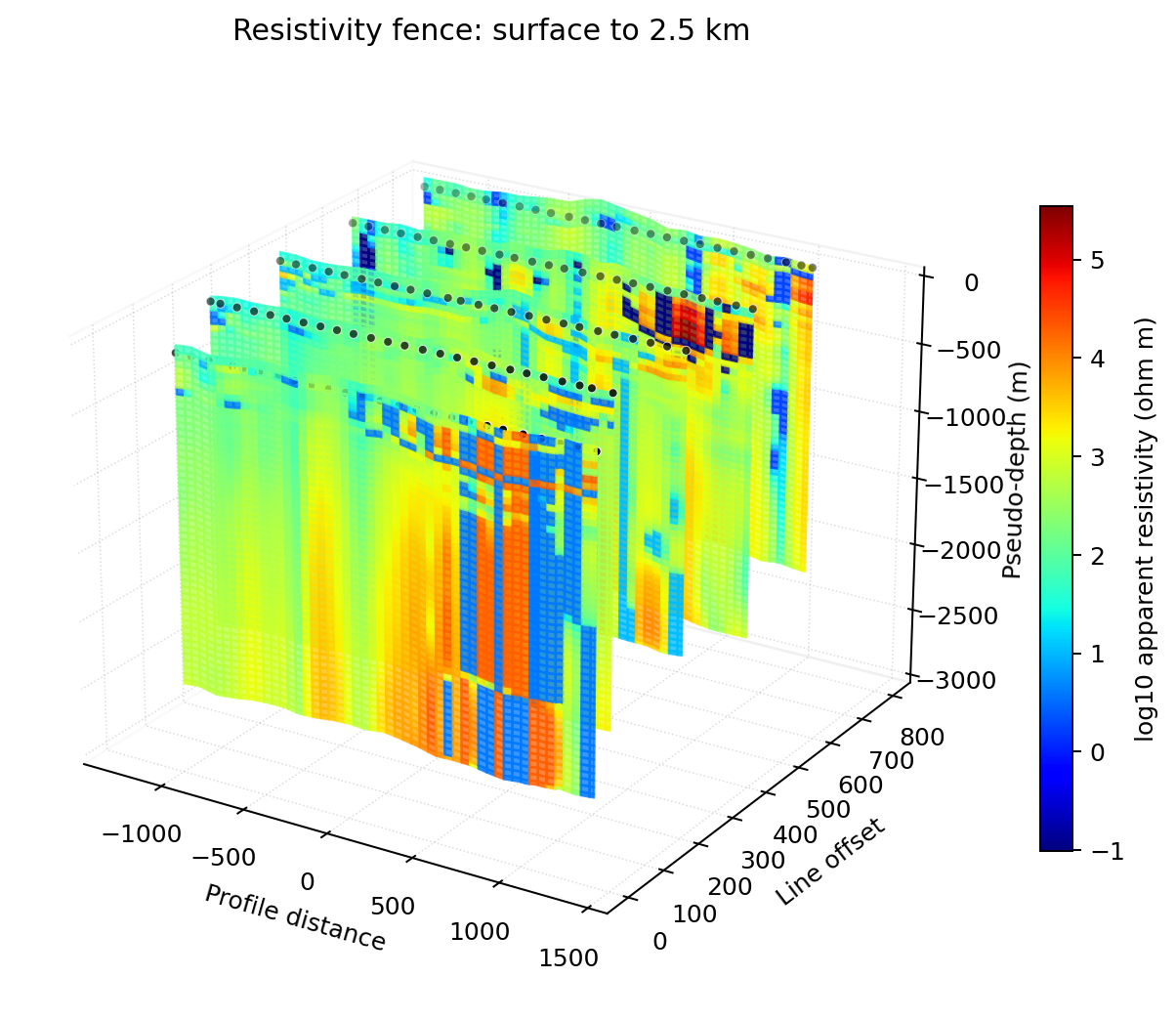
Five resistivity curtains with 0 at the top and negative
pseudo-depth downward. Surface markers retain acquisition support;
transparent panes and dotted grid lines preserve depth reference
without enclosing the data in a visually heavy box.#
Holding geometry fixed while changing the displayed quantity separates structural layout from response choice:
>>> phase = plot_volume_map(
...     data,
...     options=VolumeMapOptions(
...         mode="fence",
...         quantity="phase",
...         component="xy",
...         depth_range=(0.0, 2500.0),
...         show_stations=True,
...     ),
... )
>>> print(len(phase.data), phase.data[-1].name)
16 stations
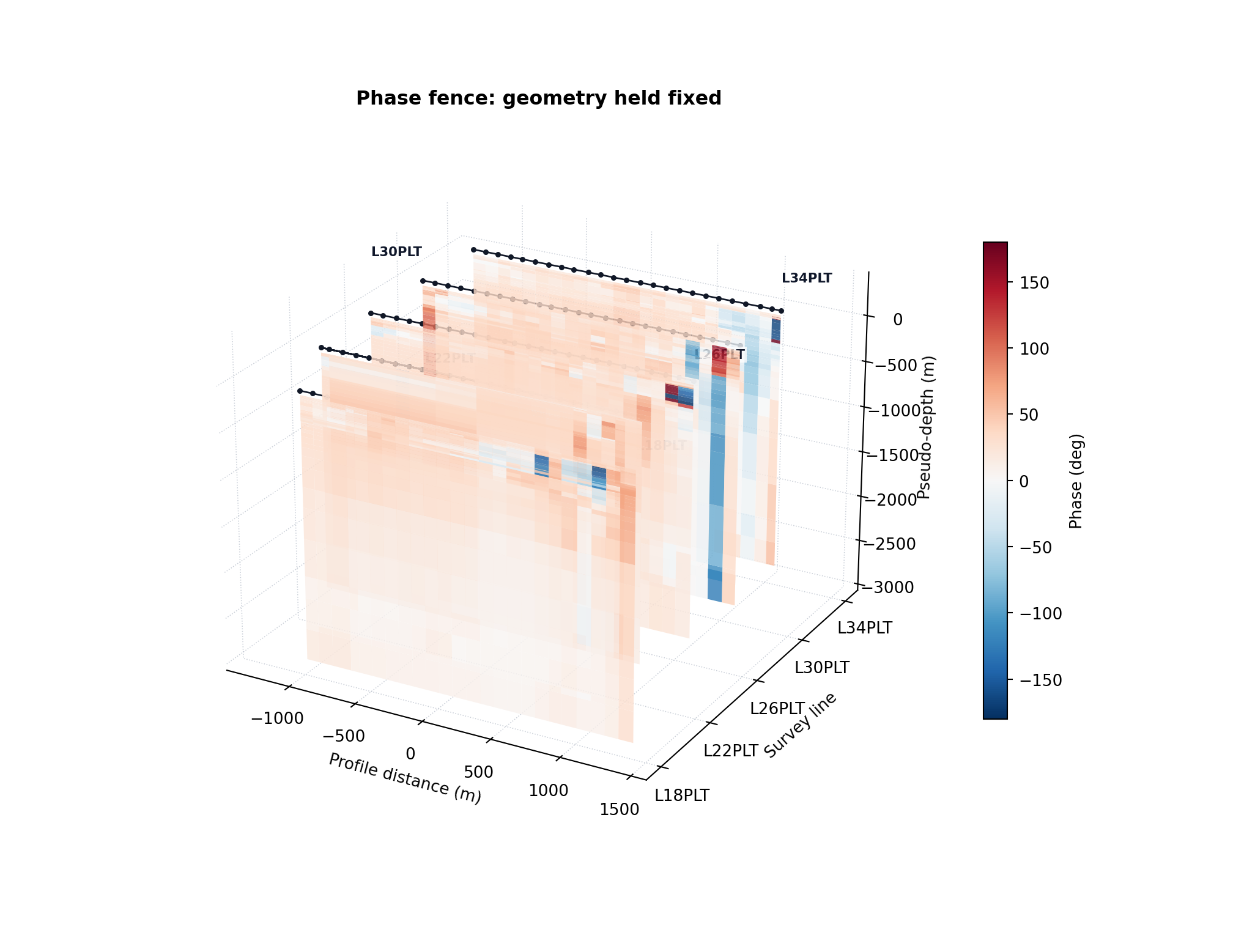
Phase colors on the same pseudo-depth geometry. Apparent resistivity
still controls the depth estimate, so this is a phase-colored
penetration-scale view rather than an independent phase-derived depth
model. Black surface tracks retain station support; the survey-line axis
and alternating endpoint annotations identify L18PLT through
L34PLT without covering the curtain interiors. Compare it with the resistivity fence to
distinguish geometry shared by construction from response patterns that
genuinely differ.#
View labeled phase-fence source codeClick to inspect and copy the complete code
 1def make_phase_fence() -> None:
 2    """Render phase curtains with station tracks and line identifiers."""
 3    data = load_lines(EDI, detect="folder", recursive=True)
 4    options = VolumeMapOptions(
 5        mode="fence", quantity="phase", component="xy",
 6        depth_range=(0.0, 3000.0), show_stations=True,
 7    )
 8    profiles = _profile_grids(data, options)
 9    norm = colors.Normalize(vmin=-180.0, vmax=180.0)
10    cmap = plt.get_cmap("RdBu_r")
11    fig = plt.figure(figsize=(10.8, 8.2), constrained_layout=True)
12    ax = fig.add_subplot(111, projection="3d")
13    for line_index, (line, grid) in enumerate(profiles.items()):
14        distance = np.asarray(grid["x"], dtype=float)
15        depth = np.asarray(grid["z"], dtype=float)
16        phase = np.asarray(grid["value"], dtype=float)
17        keep = depth <= 3000.0
18        distance, depth, phase = distance, depth[keep], phase[keep]
19        XX, ZZ = np.meshgrid(distance, -depth)
20        offset = float(line_index * 200.0)
21        YY = np.full_like(XX, offset)
22        ax.plot_surface(
23            XX, YY, ZZ, facecolors=cmap(norm(phase)),
24            shade=False, alpha=0.82, linewidth=0,
25        )
26        ax.plot(
27            distance, np.full(distance.size, offset), np.zeros(distance.size),
28            color="#111827", linewidth=1.0, marker="o", markersize=2.4,
29        )
30        endpoint = -1 if line_index % 2 == 0 else 0
31        ax.text(
32            distance[endpoint], offset, 160.0 + 38.0 * line_index,
33            line, fontsize=8, weight="bold", color="#0f172a",
34            ha="left" if endpoint == -1 else "right",
35            bbox=dict(facecolor="white", alpha=0.76,
36                      edgecolor="none", pad=1.1),
37        )
38    ax.set_title("Phase fence: geometry held fixed", weight="bold")
39    ax.set_xlabel("Profile distance (m)")
40    ax.set_ylabel("Survey line")
41    ax.set_yticks(
42        [float(index * 200.0) for index in range(len(profiles))],
43        list(profiles),
44    )
45    ax.set_zlabel("Pseudo-depth (m)")
46    ax.set_zlim(-3000.0, 400.0)
47    ax.view_init(elev=24, azim=-61)
48    ax.grid(True, linestyle=":", linewidth=0.6, alpha=0.3)
49    for axis in (ax.xaxis, ax.yaxis, ax.zaxis):
50        axis.pane.set_alpha(0.0)
51        axis._axinfo["grid"].update(
52            color=(0.39, 0.45, 0.55, 0.34),
53            linestyle=":", linewidth=0.6,
54        )
55    scalar = plt.cm.ScalarMappable(norm=norm, cmap=cmap)
56    cbar = fig.colorbar(scalar, ax=ax, shrink=0.65, pad=0.08)
57    cbar.set_label("Phase (deg)")
58    fig.savefig(IMAGES / "map_volume_phase_fence.png", dpi=190)
59    plt.close(fig)
4.4.4. Builder API#
Use pycsamt.map.VolumeMap when you want to reuse normalized
data and switch modes or quantities without reloading files.
VolumeMap is an alias of pycsamt.map.Map3D.
>>> from pycsamt.map import VolumeMap
>>> fig = (
...     VolumeMap("data/AMT/WILLY_DATA/L18PLT")
...     .with_mode("surface")
...     .with_quantity("phase")
...     .with_component("xy")
...     .figure()
... )
>>> print(len(fig.data), tuple(trace.type for trace in fig.data))
1 ('isosurface',)
The builder methods are immutable: each call returns a new builder that
shares the same MapData but carries different options.
>>> base = VolumeMap(data).with_options(
...     depth_range=(0.0, 2500.0),
...     component="xy",
... )
>>> fence = base.with_mode("fence").figure()
>>> slices = base.with_mode("depth").with_options(n_slices=6).figure()
>>> print(len(fence.data), len(slices.data))
15 11
>>> print(tuple(trace.type for trace in slices.data))
('surface', 'surface', 'surface', 'surface', 'surface', 'surface', 'scatter3d', 'scatter3d', 'scatter3d', 'scatter3d', 'scatter3d')
4.4.5. Modes#
fenceOne pseudo-depth surface per survey line. This is the best first view for multi-line surveys because it keeps each profile readable.
blockBlock volume rendering from all finite pseudo-depth samples. It is useful for a compact 3-D impression, but can hide line structure on sparse surveys.
depthHorizontal pseudo-depth slices. Values are interpolated at the slice depths generated from
depth_rangeor from the available pseudo-depth span.surfaceIsosurfaces across the pseudo-depth point cloud. Use
iso_rangeandsurface_countto control which value shells are visible.
4.4.6. Mode Examples#
Fence view with one draped surface per line:
>>> fig = plot_volume_map(
...     data,
...     options=VolumeMapOptions(
...         mode="fence",
...         quantity="resistivity",
...         component="xy",
...         show_labels=True,
...         show_contours=True,
...     ),
... )
>>> print(len(fig.data), tuple(trace.type for trace in fig.data))
15 ('surface', 'scatter3d', 'scatter3d', 'surface', 'scatter3d', 'scatter3d', 'surface', 'scatter3d', 'scatter3d', 'surface', 'scatter3d', 'scatter3d', 'surface', 'scatter3d', 'scatter3d')
>>> import numpy as np
>>> z = np.concatenate([
...     np.asarray(trace.z, dtype=float).ravel()
...     for trace in fig.data if trace.type == "surface"
... ])
>>> print(round(abs(np.nanmax(z)), 1), round(abs(np.nanmin(z)), 1))
46.4 42688.6
Block volume view:
>>> fig = plot_volume_map(
...     data,
...     options=VolumeMapOptions(
...         mode="block",
...         opacity=0.35,
...         surface_count=18,
...     ),
... )
>>> print(len(fig.data), fig.data[0].type, fig.data[0].surface.count)
1 volume 18
Depth slices:
>>> fig = plot_volume_map(
...     data,
...     options=VolumeMapOptions(
...         mode="depth",
...         depth_range=(0.0, 3000.0),
...         n_slices=7,
...         show_contours=True,
...     ),
... )
>>> surfaces = [trace for trace in fig.data if trace.type == "surface"]
>>> print(len(fig.data), len(surfaces))
12 7
>>> print([float(trace.z[0][0]) for trace in surfaces])
[-0.0, -500.0, -1000.0, -1500.0, -2000.0, -2500.0, -3000.0]
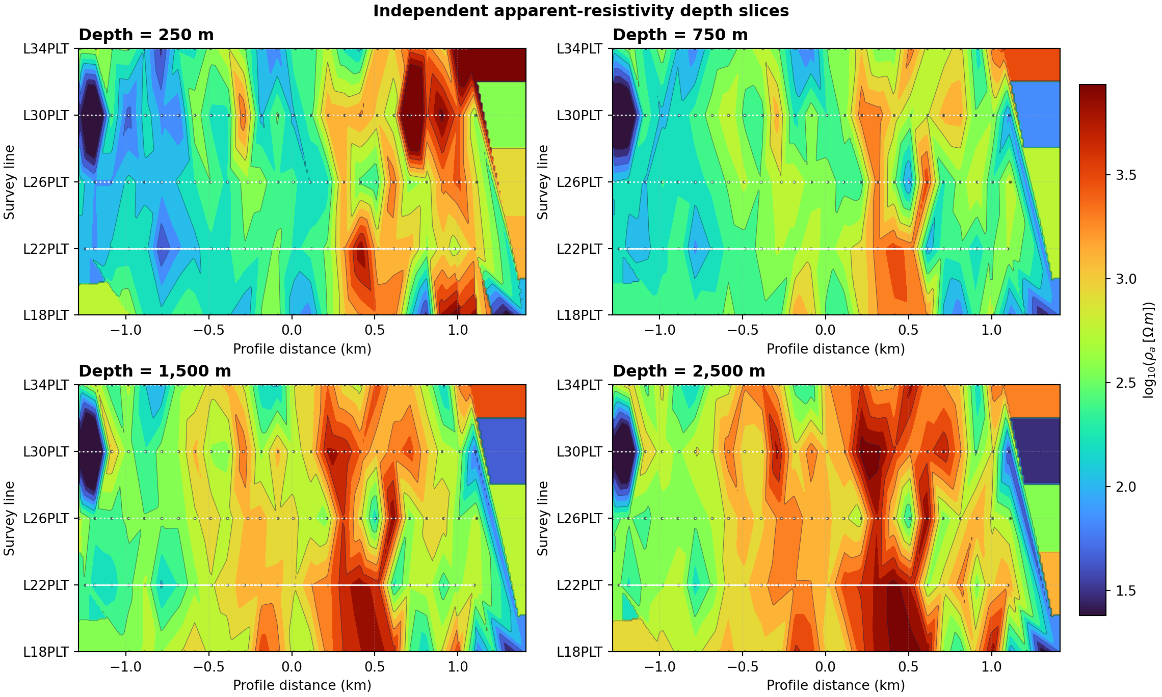
Four sampled pseudo-depth slices shown as independent contour maps. The depth is printed beside every map, and no side wall or connecting surface is drawn between adjacent levels. This separation prevents the eye from mistaking a rendering edge for a vertical anomaly. White dotted tracks and dark station points retain the five acquisition lines, while filled contours make lateral gradients between those lines easier to follow. Features between lines are interpolated and therefore have weaker support than features crossed by a station track.#
The interactive Plotly result still contains one trace per requested depth. Toggle individual traces in the legend when stacked planes obscure one another, or present them as the independent small multiples above for a static report.
View independent-depth-slice source codeClick to inspect and copy the complete code
 1def make_separated_depth_slices() -> None:
 2    """Render depth slices as independent panels with explicit depths."""
 3    data = load_lines(EDI, detect="folder", recursive=True)
 4    options = VolumeMapOptions(
 5        mode="depth",
 6        quantity="resistivity",
 7        component="xy",
 8        depth_range=(0.0, 3000.0),
 9        log_color=True,
10    )
11    profiles = _profile_grids(data, options)
12    depths = (250.0, 750.0, 1500.0, 2500.0)
13    finite = []
14    prepared = []
15    for depth in depths:
16        rows = []
17        for line, grid in profiles.items():
18            values = _values_at_depth(grid, depth, options)
19            rows.append((line, np.asarray(grid["x"]), values))
20            finite.extend(values[np.isfinite(values)])
21        prepared.append(rows)
22
23    norm = colors.Normalize(
24        vmin=np.log10(np.nanpercentile(finite, 2)),
25        vmax=np.log10(np.nanpercentile(finite, 98)),
26    )
27    fig, axes = plt.subplots(2, 2, figsize=(12.0, 7.2), constrained_layout=True)
28    levels = np.linspace(norm.vmin, norm.vmax, 15)
29    for ax, depth, rows in zip(axes.flat, depths, prepared):
30        px, py, pv = [], [], []
31        for line_index, (_line, distance, values) in enumerate(rows):
32            valid = np.isfinite(values) & (values > 0)
33            px.extend(distance[valid] / 1000.0)
34            py.extend(np.full(valid.sum(), line_index))
35            pv.extend(np.log10(values[valid]))
36        px, py, pv = map(np.asarray, (px, py, pv))
37        gx = np.linspace(px.min(), px.max(), 240)
38        gy = np.linspace(py.min(), py.max(), 150)
39        GX, GY = np.meshgrid(gx, gy)
40        # Linear interpolation respects observed gradients; nearest values
41        # only close small internal holes, while the convex-hull exterior
42        # remains masked.
43        GZ = griddata((px, py), pv, (GX, GY), method="linear")
44        nearest = griddata((px, py), pv, (GX, GY), method="nearest")
45        GZ = np.where(np.isfinite(GZ), GZ, nearest)
46        ax.contourf(
47            GX, GY, GZ, levels=levels, cmap="turbo", norm=norm,
48            extend="both",
49        )
50        ax.contour(
51            GX, GY, GZ, levels=levels[::2], colors="#172554",
52            linewidths=0.45, alpha=0.55,
53        )
54        for line_index, (_line, distance, values) in enumerate(rows):
55            valid = np.isfinite(values)
56            ax.plot(
57                distance[valid] / 1000.0,
58                np.full(valid.sum(), line_index),
59                color="white", linestyle=":", linewidth=1.15,
60                alpha=0.95,
61            )
62            ax.scatter(
63                distance[valid] / 1000.0,
64                np.full(valid.sum(), line_index),
65                s=5, color="#0f172a", alpha=0.65, linewidths=0,
66            )
67        ax.set_title(f"Depth = {depth:,.0f} m", loc="left", weight="bold")
68        ax.set_xlabel("Profile distance (km)")
69        ax.set_ylabel("Survey line")
70        ax.set_yticks(range(len(rows)), [row[0] for row in rows])
71        ax.grid(color="#94a3b8", linestyle=":", linewidth=0.7, alpha=0.45)
72        ax.set_facecolor("#f8fafc")
73    sm = plt.cm.ScalarMappable(norm=norm, cmap="turbo")
74    cbar = fig.colorbar(sm, ax=axes, shrink=0.88, pad=0.02)
75    cbar.set_label(r"$\log_{10}(\rho_a\;[\Omega\,m])$")
76    fig.suptitle("Independent apparent-resistivity depth slices", weight="bold")
77    fig.savefig(IMAGES / "map_volume_depth_slices_preview.png", dpi=190)
78    plt.close(fig)
Isosurface view:
>>> fig = plot_volume_map(
...     data,
...     options=VolumeMapOptions(
...         mode="surface",
...         iso_range=(1.0, 3.0),
...         surface_count=5,
...         opacity=0.55,
...     ),
... )
>>> print(len(fig.data), fig.data[0].type, fig.data[0].surface.count)
1 isosurface 5
The same four viewing ideas become more informative when the source is an inverted mesh rather than a pseudo-depth cloud. The following overview uses the final bundled ModEM result, which is loaded explicitly in the next part.
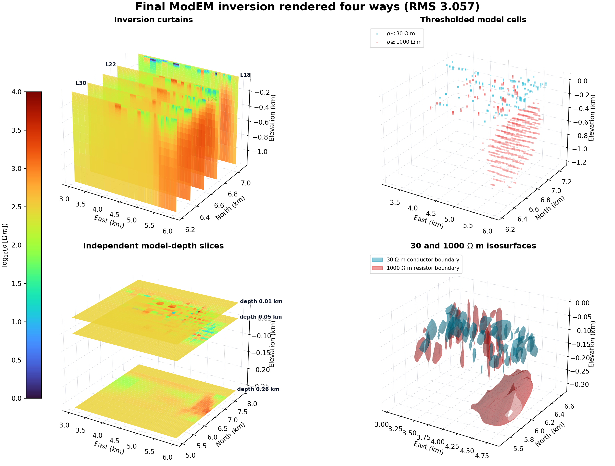
Four views of the same final ModEM inversion mesh. Curtains expose vertical changes on selected northing planes; thresholded cells isolate conductive and resistive end members; separated horizontal slices retain their model depths; and isosurfaces summarize the corresponding resistivity boundaries. Transparent panes and dotted grids retain scale without hiding the model.#
View ModEM mode-comparison source codeClick to inspect and copy the complete code
  1def make_modem_modes_overview() -> None:
  2    """Compare four views of the same final ModEM inversion model."""
  3    result, rho, x, y, z = _modem_model()
  4    # Crop padded boundary cells and the deep, very coarse mesh.  Moderate
  5    # decimation keeps the four-panel figure readable without changing the
  6    # threshold definitions.
  7    xs = x[18:-18:4] / 1000.0
  8    ys = y[5:-5:2] / 1000.0
  9    zs = z[:28] / 1000.0
 10    vol = rho[:28, 5:-5:2, 18:-18:4]
 11    log_vol = np.log10(vol)
 12    norm = colors.Normalize(0.0, 4.0)
 13    cmap = plt.get_cmap("turbo")
 14
 15    fig = plt.figure(figsize=(13.2, 10.0), constrained_layout=True)
 16
 17    # Fence: three genuine north-indexed sections through the inversion mesh.
 18    ax = fig.add_subplot(2, 2, 1, projection="3d")
 19    curtain_ax = ax
 20    XX, ZZ = np.meshgrid(xs, -zs)
 21    line_positions = {}
 22    for name, (_east, north, _height) in result.data_obs.site_coords.items():
 23        line = name.split("-")[1]
 24        line_positions.setdefault(line, []).append(north / 1000.0)
 25    model_north_origin = 0.5 * (y[0] + y[-1]) / 1000.0
 26    for line_index, (line, northings) in enumerate(
 27        sorted(line_positions.items(), key=lambda item: item[0])
 28    ):
 29        line_y = float(np.mean(northings)) + model_north_origin
 30        yi = int(np.argmin(np.abs(ys - line_y)))
 31        YY = np.full_like(XX, ys[yi])
 32        ax.plot_surface(
 33            XX, YY, ZZ, facecolors=cmap(norm(log_vol[:, yi, :])),
 34            shade=False, alpha=0.88, linewidth=0,
 35        )
 36        label_x = xs.max() + 0.04 if line_index % 2 == 0 else xs.min() - 0.04
 37        ax.text(
 38            label_x, ys[yi], -zs[0] - 0.012 * line_index, f"L{line}",
 39            fontsize=8, weight="bold", color="#0f172a",
 40            ha="left" if line_index % 2 == 0 else "right",
 41            bbox=dict(facecolor="white", alpha=0.72, edgecolor="none", pad=1.2),
 42        )
 43    ax.set_title("Inversion curtains", weight="bold")
 44    _light_3d_frame(ax)
 45
 46    # Block: retain only interpretable end members instead of an opaque cube.
 47    ax = fig.add_subplot(2, 2, 2, projection="3d")
 48    for mask, color, label in (
 49        (vol <= 30.0, "#06b6d4", r"$\rho\leq30$ $\Omega$ m"),
 50        (vol >= 1000.0, "#ef4444", r"$\rho\geq1000$ $\Omega$ m"),
 51    ):
 52        zi, yi, xi = np.nonzero(mask)
 53        stride = max(1, zi.size // 1800 + 1)
 54        ax.scatter(
 55            xs[xi[::stride]], ys[yi[::stride]], -zs[zi[::stride]],
 56            s=5, marker="s", color=color, alpha=0.28,
 57            linewidths=0, label=label,
 58        )
 59    ax.set_title("Thresholded model cells", weight="bold")
 60    ax.legend(loc="upper left", fontsize=8)
 61    _light_3d_frame(ax)
 62
 63    # Depth: independent horizontal surfaces with a small vertical gap.
 64    ax = fig.add_subplot(2, 2, 3, projection="3d")
 65    depth_ax = ax
 66    XI, YI = np.meshgrid(xs, ys)
 67    for zi in (5, 12, 20):
 68        plane = log_vol[zi]
 69        ax.plot_surface(
 70            XI, YI, np.full_like(XI, -zs[zi]),
 71            facecolors=cmap(norm(plane)), shade=False,
 72            alpha=0.86, linewidth=0,
 73        )
 74        ax.text(
 75            xs.max() + 0.04, ys.max(), -zs[zi],
 76            f"depth {zs[zi]:.2f} km", fontsize=8, weight="bold",
 77            color="#0f172a",
 78            bbox=dict(facecolor="white", alpha=0.78, edgecolor="none", pad=1.2),
 79        )
 80    ax.set_title("Independent model-depth slices", weight="bold")
 81    _light_3d_frame(ax)
 82
 83    # Surface: explicit conductive and resistive boundaries.
 84    ax = fig.add_subplot(2, 2, 4, projection="3d")
 85    spacing = (
 86        float(np.median(np.diff(zs))),
 87        float(np.median(np.diff(ys))),
 88        float(np.median(np.diff(xs))),
 89    )
 90    for level, color in ((np.log10(30.0), "#0891b2"),
 91                         (np.log10(1000.0), "#dc2626")):
 92        verts, faces, _, _ = marching_cubes(log_vol, level=level, spacing=spacing)
 93        ax.plot_trisurf(
 94            verts[:, 2] + xs.min(), verts[:, 1] + ys.min(), -verts[:, 0],
 95            triangles=faces, color=color, alpha=0.32,
 96            linewidth=0.04, edgecolor=color,
 97        )
 98    ax.set_title("30 and 1000 $\Omega$ m isosurfaces", weight="bold")
 99    ax.legend(
100        handles=[
101            Patch(color="#0891b2", alpha=0.45,
102                  label=r"30 $\Omega$ m conductor boundary"),
103            Patch(color="#dc2626", alpha=0.45,
104                  label=r"1000 $\Omega$ m resistor boundary"),
105        ],
106        loc="upper left", fontsize=8,
107    )
108    _light_3d_frame(ax)
109
110    scalar = plt.cm.ScalarMappable(norm=norm, cmap=cmap)
111    cbar = fig.colorbar(
112        scalar, ax=[curtain_ax, depth_ax], shrink=0.7,
113        pad=0.02, location="left",
114    )
115    cbar.set_label(r"$\log_{10}(\rho\;[\Omega\,m])$")
116    fig.suptitle(
117        f"Final ModEM inversion rendered four ways (RMS {result.final_rms:.3f})",
118        fontsize=17, weight="bold",
119    )
120    fig.savefig(IMAGES / "map_volume_modes_overview.png", dpi=190)
121    plt.close(fig)
For EDI input, fence preserves measured line topology most directly, while block and isosurface views require cross-line interpolation. In the figure above, however, every panel samples a genuine inversion mesh; changing the view changes which cells or boundaries are exposed, not the underlying resistivity solution. Rendering continuity still must not be confused with model resolution.
4.4.7. ModEM Inversion Volumes#
The preceding EDI examples use pseudo-depth. A ModEM .rho result is
different: it is an inverted resistivity mesh with explicit east, north,
and depth cells. The bundled Willy result can be loaded together with its
matching response file, and pycsamt.map.load_modem_lines() selects the
latest compatible pair automatically.
>>> from pycsamt.map import load_modem_lines
>>> inversion = load_modem_lines(
...     "data/modem/willy_27freq_watex_line02_sample",
...     fetch_elevation=False,
... )
>>> print(inversion.lines)
('18', '22', '26', '30', '34')
>>> print(len(inversion.stations), inversion.metadata["rms"])
125 3.057151
>>> print({
...     line: section["rho"].shape
...     for line, section in inversion.metadata["sections"].items()
... })
{'18': (41, 25), '22': (41, 25), '26': (41, 25), '30': (41, 25), '34': (41, 25)}
These arrays are vertical curtains sampled through the inversion mesh at the ModEM stations. They bypass the skin-depth calculation in (2); consequently their vertical coordinates are model cell depths and their colors are inverted resistivity.
A threshold turns the full range into a target-oriented view. Here the conductive block retains only cells at or below 30 ohm metres:
>>> conductive = plot_volume_map(
...     inversion,
...     options=VolumeMapOptions(
...         mode="block",
...         rho_range=(0.01, 30.0),
...         value_range=(0.01, 30.0),
...         log_color=True,
...         opacity=0.25,
...         surface_count=18,
...     ),
... )
>>> print(len(conductive.data), conductive.data[0].type)
1 volume
The complementary resistive view uses rho_range=(1000.0, 10000.0).
Showing both thresholds separately is normally clearer than allowing the
resistive background to hide a compact conductor.
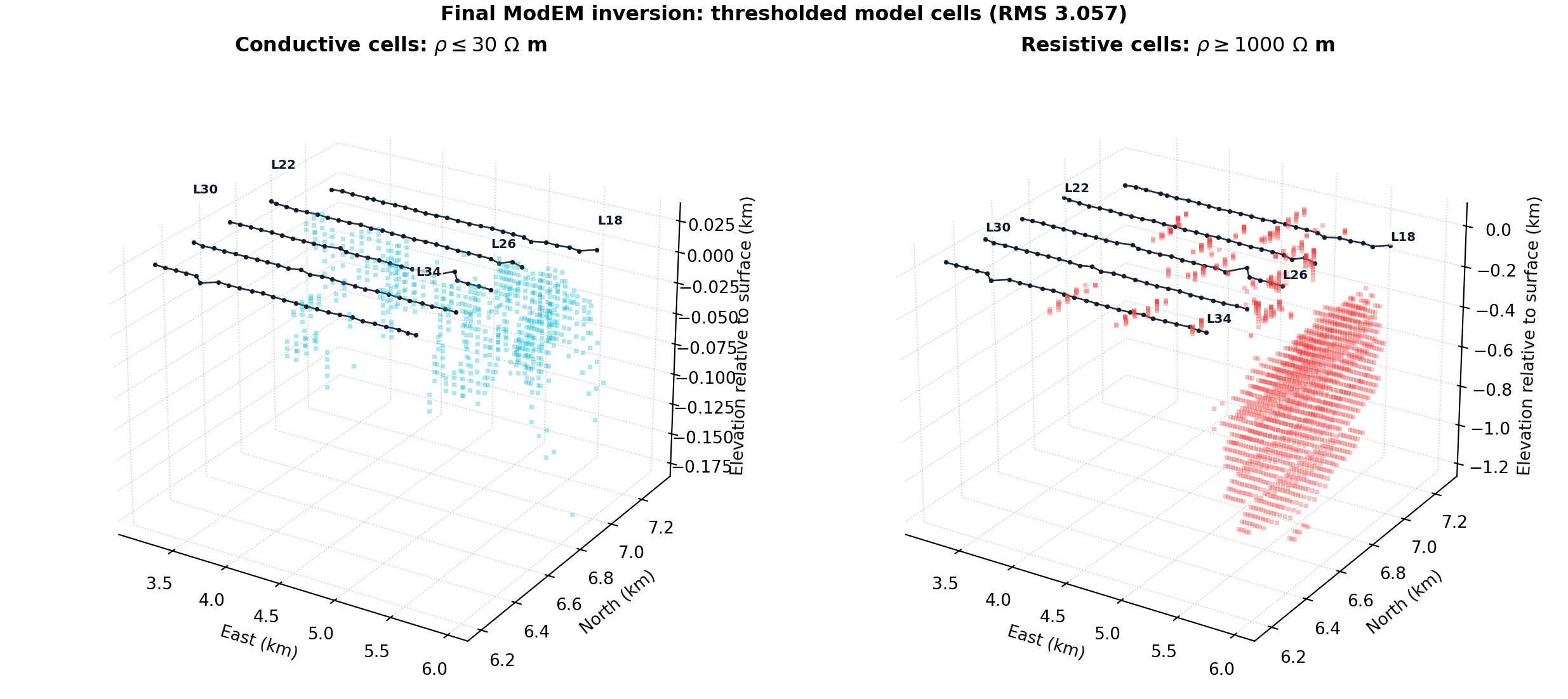
Thresholded cells from the final inversion model. Cyan identifies the shallow, discontinuous volume at or below 30 ohm metres; red identifies cells at or above 1000 ohm metres, including the more continuous body on the eastern side. Black surface tracks and labels locate lines L18, L22, L26, L30, and L34 above both threshold classes. Thresholds define visualization classes, not unique lithologies, and should be interpreted with sensitivity, resolution, and geological constraints.#
View ModEM threshold-volume source codeClick to inspect and copy the complete code
 1def make_modem_threshold_blocks() -> None:
 2    """Show conductive and resistive cells from the final ModEM model."""
 3    result, rho, x, y, z = _modem_model()
 4    # Remove the laterally padded boundary and deepest coarse cells, then
 5    # decimate the long x direction to keep individual voxels legible.
 6    volume = rho[:28, 5:-5, 18:-18:4]
 7    xx = x[18:-18:4] / 1000.0
 8    yy = y[5:-5] / 1000.0
 9    zz = z[:28] / 1000.0
10    X, Y, Z = np.meshgrid(xx, yy, zz, indexing="xy")
11    station_lines = {}
12    x_origin = 0.5 * (x[0] + x[-1]) / 1000.0
13    y_origin = 0.5 * (y[0] + y[-1]) / 1000.0
14    for name, (east, north, _height) in result.data_obs.site_coords.items():
15        line = name.split("-")[1]
16        station_lines.setdefault(line, []).append(
17            (east / 1000.0 + x_origin, north / 1000.0 + y_origin)
18        )
19
20    fig = plt.figure(figsize=(13.0, 5.8), constrained_layout=True)
21    cases = ((30.0, "Conductive cells: $\\rho \\leq 30$ $\\Omega$ m", "#06b6d4"),
22             (1000.0, "Resistive cells: $\\rho \\geq 1000$ $\\Omega$ m", "#ef4444"))
23    for index, (threshold, title, color) in enumerate(cases, start=1):
24        ax = fig.add_subplot(1, 2, index, projection="3d")
25        mask = volume <= threshold if index == 1 else volume >= threshold
26        zi, yi, xi = np.nonzero(mask)
27        values = volume[mask]
28        keep = np.arange(values.size) % max(1, values.size // 3500 + 1) == 0
29        ax.scatter(
30            xx[xi[keep]], yy[yi[keep]], -zz[zi[keep]],
31            c=color, s=7, marker="s", alpha=0.32, linewidths=0,
32        )
33        for line_index, (line, points) in enumerate(sorted(station_lines.items())):
34            points = np.asarray(points)
35            order = np.argsort(points[:, 0])
36            points = points[order]
37            ax.plot(
38                points[:, 0], points[:, 1], np.full(points.shape[0], 0.025),
39                color="#111827", linewidth=1.0, marker="o", markersize=1.8,
40                alpha=0.9,
41            )
42            endpoint = -1 if line_index % 2 == 0 else 0
43            ax.text(
44                points[endpoint, 0], points[endpoint, 1],
45                0.045 + 0.006 * line_index, f"L{line}",
46                fontsize=7.5, weight="bold", color="#0f172a",
47                bbox=dict(facecolor="white", alpha=0.72,
48                          edgecolor="none", pad=1.0),
49            )
50        ax.set_title(title, weight="bold")
51        ax.set_xlabel("East (km)")
52        ax.set_ylabel("North (km)")
53        ax.set_zlabel("Elevation relative to surface (km)")
54        ax.grid(True, linestyle=":", linewidth=0.65, alpha=0.32)
55        ax.xaxis.pane.set_alpha(0.0)
56        ax.yaxis.pane.set_alpha(0.0)
57        ax.zaxis.pane.set_alpha(0.0)
58        for axis in (ax.xaxis, ax.yaxis, ax.zaxis):
59            axis._axinfo["grid"].update(
60                color=(0.39, 0.45, 0.55, 0.35),
61                linestyle=":",
62                linewidth=0.65,
63            )
64        ax.view_init(elev=25, azim=-58)
65    fig.suptitle(
66        f"Final ModEM inversion: thresholded model cells (RMS {result.final_rms:.3f})",
67        weight="bold",
68    )
69    fig.savefig(IMAGES / "map_volume_modem_threshold_blocks.png", dpi=190)
70    plt.close(fig)
An isosurface replaces the visible cells by a boundary at a chosen
resistivity. For logarithmic colors, iso_range is expressed in
\(\log_{10}\) space, whereas rho_range remains in physical units:
>>> conductor_shell = plot_volume_map(
...     inversion,
...     options=VolumeMapOptions(
...         mode="surface",
...         rho_range=(0.01, 30.0),
...         iso_range=(-2.0, 1.4771212547),
...         log_color=True,
...         surface_count=4,
...         opacity=0.35,
...     ),
... )
>>> shell = conductor_shell.data[0]
>>> print(shell.type, shell.surface.count, shell.isomin, round(shell.isomax, 3))
isosurface 4 -2.0 1.477
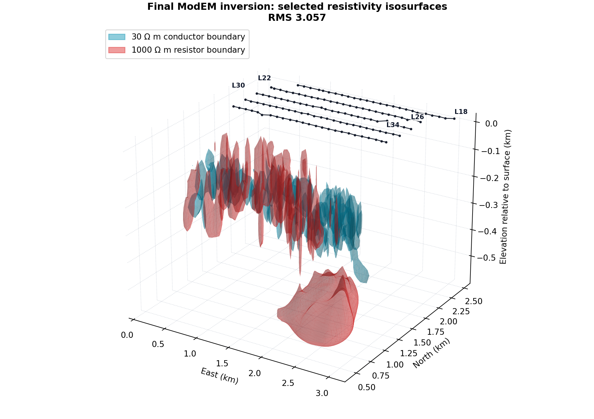
The 30-ohm-metre and 1000-ohm-metre boundaries reveal body continuity more clearly than opaque blocks. Black surface tracks, station markers, and labels locate lines L18 through L34 above the shells. Overlap in projection does not mean that one cell satisfies both thresholds: each translucent shell marks a different crossing of the continuous rendering field. Rotate the HTML figure and inspect each shell independently before assigning geometry.#
View ModEM isosurface source codeClick to inspect and copy the complete code
 1def make_modem_isosurfaces() -> None:
 2    """Extract conductive and resistive boundaries with marching cubes."""
 3    result, rho, x, y, z = _modem_model()
 4    log_rho = np.log10(rho[:32, 4:-4, 12:-12])
 5    spacing = (
 6        float(np.median(np.diff(z[:32]))) / 1000.0,
 7        float(np.median(np.diff(y[4:-4]))) / 1000.0,
 8        float(np.median(np.diff(x[12:-12]))) / 1000.0,
 9    )
10    fig = plt.figure(figsize=(10.2, 7.2), constrained_layout=True)
11    ax = fig.add_subplot(111, projection="3d")
12    for level, color, label in (
13        (np.log10(30.0), "#0891b2", r"30 $\Omega$ m conductor boundary"),
14        (np.log10(1000.0), "#dc2626", r"1000 $\Omega$ m resistor boundary"),
15    ):
16        verts, faces, _, _ = marching_cubes(log_rho, level=level, spacing=spacing)
17        # marching_cubes returns coordinates in (z, y, x) order.
18        ax.plot_trisurf(
19            verts[:, 2], verts[:, 1], -verts[:, 0],
20            triangles=faces, color=color, alpha=0.28,
21            linewidth=0.05, edgecolor=color,
22        )
23    x_origin = 0.5 * (x[0] + x[-1]) / 1000.0 - x[12] / 1000.0
24    y_origin = 0.5 * (y[0] + y[-1]) / 1000.0 - y[4] / 1000.0
25    station_lines = {}
26    for name, (east, north, _height) in result.data_obs.site_coords.items():
27        line = name.split("-")[1]
28        station_lines.setdefault(line, []).append(
29            (east / 1000.0 + x_origin, north / 1000.0 + y_origin)
30        )
31    for line_index, (line, points) in enumerate(sorted(station_lines.items())):
32        points = np.asarray(points)
33        order = np.argsort(points[:, 0])
34        points = points[order]
35        ax.plot(
36            points[:, 0], points[:, 1], np.full(points.shape[0], 0.018),
37            color="#111827", linewidth=1.05, marker="o", markersize=2.0,
38            alpha=0.92,
39        )
40        endpoint = -1 if line_index % 2 == 0 else 0
41        ax.text(
42            points[endpoint, 0], points[endpoint, 1],
43            0.035 + 0.009 * line_index, f"L{line}",
44            fontsize=8, weight="bold", color="#0f172a",
45            ha="left" if endpoint == -1 else "right",
46            bbox=dict(facecolor="white", alpha=0.76,
47                      edgecolor="none", pad=1.0),
48        )
49    ax.set_xlabel("East (km)")
50    ax.set_ylabel("North (km)")
51    ax.set_zlabel("Elevation relative to surface (km)")
52    ax.set_title(
53        f"Final ModEM inversion: selected resistivity isosurfaces\nRMS {result.final_rms:.3f}",
54        weight="bold",
55    )
56    ax.grid(True, linestyle=":", linewidth=0.65, alpha=0.3)
57    ax.xaxis.pane.set_alpha(0.0)
58    ax.yaxis.pane.set_alpha(0.0)
59    ax.zaxis.pane.set_alpha(0.0)
60    for axis in (ax.xaxis, ax.yaxis, ax.zaxis):
61        axis._axinfo["grid"].update(
62            color=(0.39, 0.45, 0.55, 0.35),
63            linestyle=":",
64            linewidth=0.65,
65        )
66    ax.view_init(elev=24, azim=-58)
67    ax.legend(
68        handles=[
69            Patch(color="#0891b2", alpha=0.45,
70                  label=r"30 $\Omega$ m conductor boundary"),
71            Patch(color="#dc2626", alpha=0.45,
72                  label=r"1000 $\Omega$ m resistor boundary"),
73        ],
74        loc="upper left",
75    )
76    fig.savefig(IMAGES / "map_volume_modem_isosurfaces.png", dpi=190)
77    plt.close(fig)
4.4.8. Filtering#
depth_range clips the pseudo-depth axis. period_range filters
the periods before grid construction. rho_range masks samples by
apparent resistivity, even when the displayed quantity is phase.
iso_range controls the value range used by isosurface rendering.
Use value_range to keep colorbars comparable across multiple
figures:
>>> options = VolumeMapOptions(
...     mode="fence",
...     quantity="resistivity",
...     log_color=True,
...     value_range=(10.0, 10000.0),
...     rho_range=(10.0, 10000.0),
...     period_range=(0.001, 5.0),
...     depth_range=(0.0, 2500.0),
... )
>>> filtered = plot_volume_map(data, options=options)
>>> surfaces = [trace for trace in filtered.data if trace.type == "surface"]
>>> print(len(surfaces), surfaces[0].cmin, surfaces[0].cmax)
5 1.0 4.0
rho_range filters in physical apparent-resistivity units. When
log_color=True, value_range is converted to log10 color space
for resistivity colorbars.
The filter order is worth keeping explicit in scripts. period_range
removes rows before pseudo-depth grids are built. depth_range clips
the resulting \(z_j\) values. rho_range masks cells whose
physical apparent resistivity falls outside the requested interval. If
log_color=True, only the displayed color values are transformed to
\(\log_{10}(\rho_a)\); the depth estimate and rho_range filter
stay in physical units.
The masking consequence is easier to see on a single curtain:
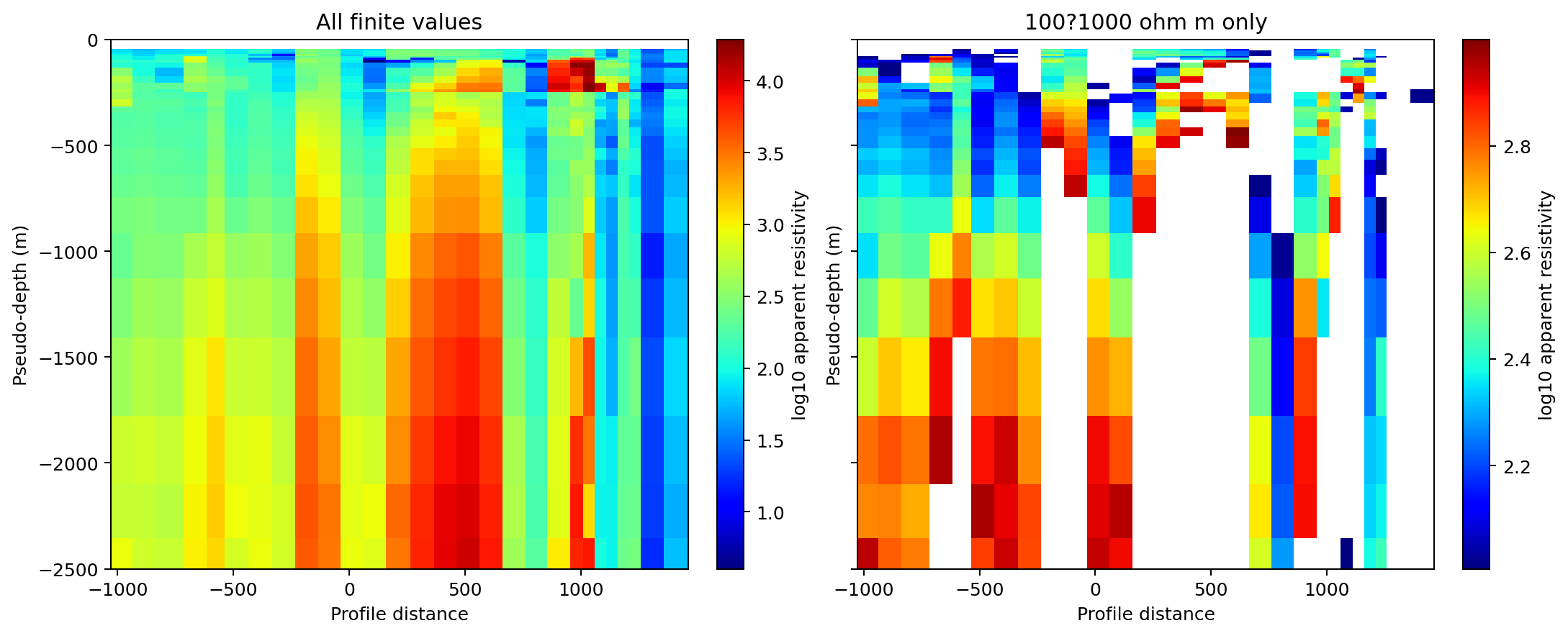
The same L18 section before and after retaining only 100–1000
ohm-metre cells. White gaps in the filtered view are deliberately
excluded values, not missing stations or transparent geological
bodies. Archive the physical rho_range with the figure.#
4.4.9. Components#
The component option selects the impedance component used to build
the pseudosection table:
"xy","yx","xx","yy"Individual tensor components.
"avg"Average of
xyandyx."det"Determinant-style derived value for resistivity, or average phase.
Use the same component for volume maps that you use in profile pseudosections when you want the 2-D and 3-D views to compare directly.
4.4.10. Line Spacing And Azimuth#
line_spacing controls the offset between profile lines in the 3-D
scene. azimuth rotates those line offsets.
>>> fig = plot_volume_map(
...     data,
...     options=VolumeMapOptions(
...         mode="fence",
...         line_spacing=1.5,
...         azimuth=30.0,
...     ),
... )
>>> print(len(fig.data), tuple(trace.type for trace in fig.data[:3]))
15 ('surface', 'scatter3d', 'scatter3d')
With azimuth=0, line offsets appear along the scene y axis.
With azimuth=90, offsets are shifted into the x direction.
For a line offset \(d_\ell\) and azimuth \(\alpha\), the plotted
coordinates are
Equation (3) changes scene placement for fence and depth views. Block mode deliberately remains axis-aligned because Plotly volume reconstruction requires a rectilinear grid.
4.4.11. Topography And Terrain#
By default, depth is plotted downward from a flat surface. Enable
topography to use station elevations from the loaded EDI metadata:
>>> fig = plot_volume_map(
...     data,
...     options=VolumeMapOptions(
...         mode="fence",
...         topography=True,
...         show_terrain=True,
...     ),
... )
>>> print(fig.layout.scene.zaxis.title.text)
Elevation - depth (m)
>>> print(len(fig.data), tuple(trace.type for trace in fig.data[:3]))
15 ('surface', 'scatter3d', 'scatter3d')
When topography=True, the vertical axis is labelled
Elevation - depth (m) and each pseudo-depth surface is shifted by
the station elevations. show_terrain=True adds a terrain trace at
the top of each line. If elevations are missing, zeros are used for
those stations.
With topography enabled, a displayed vertical coordinate is \(z' = h_i - z_j\), where \(h_i\) is station elevation and \(z_j\) is pseudo-depth. With topography disabled, \(h_i=0\) for every station.
4.4.12. Station Markers#
Set show_stations=True to add station markers at the survey
surface.
>>> fig = plot_volume_map(
...     data,
...     options=VolumeMapOptions(
...         mode="fence",
...         show_stations=True,
...         station_symbol="diamond",
...         station_size=5,
...         station_color="#111827",
...     ),
... )
>>> print(len(fig.data), fig.data[-1].type, fig.data[-1].name)
16 scatter3d stations
Markers use the same line offsets and optional topography shift as the volume surfaces.
4.4.13. Color And Theme Controls#
Volume maps support the shared map themes and Plotly color scales:
>>> fig = plot_volume_map(
...     data,
...     options=VolumeMapOptions(
...         mode="depth",
...         theme="dark",
...         cmap="Turbo",
...         opacity=0.75,
...         title="Depth slices: XY resistivity",
...     ),
... )
>>> print(fig.layout.title.text, fig.data[0].opacity)
Depth slices: XY resistivity 0.75
For resistivity, log_color=True is the default. For phase, values
are shown linearly and the colorbar title becomes Phase (deg).
4.4.14. Exporting 3-D Views#
HTML is the safest export for 3-D Plotly figures because it preserves rotation, zoom, hover labels, and all surfaces:
>>> from pycsamt.map import write_html
>>> output = write_html(fig, "outputs/volume_depth.html")
>>> print(output.as_posix())
outputs/volume_depth.html
Static image export is possible when a Plotly image backend such as Kaleido is installed:
>>> from pycsamt.map import save_png
>>> output = save_png(
...     fig,
...     "outputs/volume_depth.png",
...     width=1600,
...     height=1000,
... )
>>> print(output.as_posix())
outputs/volume_depth.png
4.4.15. Troubleshooting#
- Empty 3-D figure
No pseudosection rows could be built. Check that stations have a valid
Zobject with frequency, resistivity, and phase arrays.- Only one line appears
Line metadata may be missing. Use
pycsamt.map.load_lines()with an explicit mapping ordetect="folder"before plotting.- Depth range removes everything
The pseudo-depth estimate may be outside your requested
depth_range. Temporarily remove the range and inspect the full extent.- Phase map still responds to
rho_range This is expected. Apparent resistivity is still used to estimate pseudo-depth and to apply resistivity masks.
- Isosurfaces look empty
iso_rangemay not overlap the color-space values. For resistivity withlog_color=True, use log10 values iniso_range.- Terrain is flat
Elevations may be missing or non-finite. The terrain shift uses station elevations from the normalized
StationRecordobjects.