
11.10. Skew Diagnostics#
pycsamt.emtools.skew documents how far an impedance tensor departs
from a simple 1-D or 2-D response. It gives two complementary views of
skew:
Bahr skewness, written \(\eta\), computed directly from the complex impedance tensor
Z.Phase-tensor skew, written \(\beta\), computed through the phase-tensor table and reported in degrees.
Use skew diagnostics before 2-D preparation, dimensionality
decisions, strike interpretation, frequency masking, and inversion
setup. A low skew band supports a 1-D/2-D approximation. A high skew
band warns that the tensor may contain 3-D structure,
galvanic distortion, local noise, or component geometry that
should not be forced into a simple 2-D workflow without more checks.
Every example below uses pyCSAMT’s bundled AMT line,
data/AMT/WILLY_DATA/L18PLT – a genuinely high-skew survey, as the
numbers throughout this page will show.
Full signatures and parameter defaults are maintained in the
API reference. This page explains how to use
the public workflow functions through pycsamt.emtools.
11.10.1. Two Skew Measures#
Bahr skewness is computed from impedance invariants. In pyCSAMT it is
available through bahr_skewness and accepts either a tensor block of
shape (n_freq, 2, 2) or a flattened block of shape (n_freq, 4).
It is exactly the Bahr skewness glossary formula,
Phase-tensor skew starts from the phase tensor itself, built from the real and imaginary parts of the same impedance tensor,
and the skew angle is then the Caldwell-Bibby-Bahr invariant, with \(\Phi = \begin{pmatrix}\Phi_{xx} & \Phi_{xy}\\ \Phi_{yx} & \Phi_{yy}\end{pmatrix}\),
reported in degrees – the same \(\beta\) the skew glossary
entry defines, and rotation-invariant unlike the companion orientation
angle \(\alpha = \tfrac{1}{2}\operatorname{atan2}(\Phi_{xy} +
\Phi_{yx},\ \Phi_{xx} - \Phi_{yy})\) that build_phase_tensor_table
also returns. skew_table returns the same table produced by the
phase-tensor workflow, including station, freq, period,
beta, and skew – in this module skew is just an alias for
beta, kept because that is the column name the masking and voting
helpers below were written against.
The two measures are related but not interchangeable. Bahr
\(\eta\) is a direct invariant of Z. Phase-tensor
\(\beta\) depends on the real and imaginary impedance parts through
the phase tensor. They can agree that a station is non-2-D while ranking
the severity differently.
11.10.2. Workflow Map#
Goal |
Use this |
Result |
|---|---|---|
Compute a station-frequency skew table |
|
A |
Compute Bahr skew from a Z block |
|
A one-dimensional array of \(\eta\) values. |
Mask rows above a skew threshold |
|
A |
Keep one contiguous low-skew run per station |
|
A station-wise band mask. |
Bridge short gaps inside low-skew runs |
|
A less fragmented station-wise mask. |
Keep a survey-wide low-skew band |
|
A shared frequency band selected by station vote. |
Plot skew quality across the line |
|
Pseudo-section, period ribbon, and vote-curve views. |
Plot Bahr skew for one station |
|
A single-station \(\eta\) plot against a threshold. |
11.10.3. Loading The Survey#
Load once with ensure_sites and reuse the same raw object for
diagnostics and before/after checks.
>>> from pathlib import Path
>>> from pycsamt.emtools import ensure_sites
>>> edi_dir = Path("data/AMT/WILLY_DATA/L18PLT")
>>> sites = ensure_sites(edi_dir, recursive=True, verbose=0)
Most masking functions default to inplace=False. That means the
returned Sites object is masked, while sites remains available
for comparison.
11.10.4. Phase-Tensor Skew Table#
Start with skew_table. It summarizes \(\beta\) at every
station-frequency row.
>>> from pycsamt.emtools import ensure_sites, skew_table
>>> sites = ensure_sites("data/AMT/WILLY_DATA/L18PLT", recursive=True)
>>> table = skew_table(sites)
>>> table.columns
Index(['station', 'freq', 'period', 's1', 's2', 'theta', 'alpha', 'beta',
       'skew', 'ellipt'],
      dtype='object')
>>> table[["station", "freq", "period", "beta", "skew"]].head()
   station     freq    period      beta      skew
0  18-001A  10400.0  0.000096  2.611588  2.611588
1  18-001A   8707.0  0.000115  1.964321  1.964321
2  18-001A   7289.0  0.000137  1.804266  1.804266
3  18-001A   6102.0  0.000164  1.068855  1.068855
4  18-001A   5108.0  0.000196 -6.949269 -6.949269
>>> table["skew"].abs().describe()
count    1484.000000
mean       23.850491
std        23.490731
min         0.050944
25%         5.375451
50%        14.920270
75%        37.654544
max        89.811834
Name: skew, dtype: float64
>>> station_summary = (
...     table.assign(abs_skew=table["skew"].abs())
...     .groupby("station", as_index=False)
...     .agg(
...         n_freq=("freq", "size"),
...         median_abs_skew=("abs_skew", "median"),
...         max_abs_skew=("abs_skew", "max"),
...     )
...     .sort_values("median_abs_skew")
... )
>>> station_summary.head()
    station  n_freq  median_abs_skew  max_abs_skew
0   18-001A      53         4.809977     88.625613
1   18-002U      53         6.596544     54.370326
6   18-007U      53         8.377503     54.171200
11  18-012A      53         9.052529     82.530092
7   18-008U      53         9.136982     81.792497
>>> station_summary.tail()
    station  n_freq  median_abs_skew  max_abs_skew
19  18-020A      53        45.539049     84.467238
21  18-021U      53        46.582007     79.328230
20  18-021B      53        47.235914     89.119132
22  18-022U      53        49.751057     89.263622
24  18-023A      53        54.529465     88.439189
Interpret skew and beta as angles in degrees. A common strict
phase-tensor threshold is around 3 to 6 degrees. This line sits
well above it: median absolute skew across all 1484 station-frequency
rows is nearly 15 degrees, and the top quartile runs past 37.
The two ends of station_summary also line up with where a station
sits along the profile – the lowest-skew stations are all in the
18-001A-18-012A range, while every station from 18-020A
onward lands in the highest-skew tail. When most of a survey clears a
strict threshold by this much, do not blindly mask the whole line.
First inspect the distribution and decide whether the threshold is
appropriate for the question being asked.
11.10.5. Bahr Skewness#
Use bahr_skewness when you want an independent skew measure computed
directly from impedance.
>>> import numpy as np
>>> from pycsamt.emtools import bahr_skewness, ensure_sites
>>> sites = ensure_sites("data/AMT/WILLY_DATA/L18PLT", recursive=True)
>>> station = next(iter(sites))
>>> z = station.z
>>> freq = station.freq
>>> eta = bahr_skewness(z)
>>> period = 1.0 / freq
>>> print(np.nanmin(eta), np.nanmedian(eta), np.nanmax(eta))
0.8461749951030751 1.5856487464775848 2.9879890035270154
>>> print(period[:5], eta[:5])
[9.61538462e-05 1.14850121e-04 1.37193031e-04 1.63880695e-04
 1.95771339e-04] [2.97741225 2.987989   2.86896122 2.57559637 2.18481788]
The classic Bahr threshold often used as a 2-D/3-D guide is
eta = 0.4. Every one of this station’s printed values sits well
above it – even the minimum, 0.85, is more than double the
threshold. Treat that boundary as a diagnostic aid, not an automatic
editing rule. Large \(\eta\) can reflect genuine 3-D structure, but
it can also reflect noise, distortion, or component problems.
11.10.6. Bahr Skew Plot#
plot_skewness plots Bahr \(\eta\) against log-period and draws
the threshold line.
>>> import matplotlib.pyplot as plt
>>> from pycsamt.emtools import ensure_sites, plot_skewness
>>> sites = ensure_sites("data/AMT/WILLY_DATA/L18PLT", recursive=True)
>>> station = next(iter(sites))
>>> fig, ax = plt.subplots(figsize=(7, 4))
>>> _ = plot_skewness(
...     station.freq,
...     station.z,
...     threshold=0.4,
...     ax=ax,
...     title=str(getattr(station, "name", "station")),
... )
>>> fig.tight_layout()
>>> fig.savefig("bahr_skewness_18-001A.png", dpi=200)
>>> plt.close(fig)
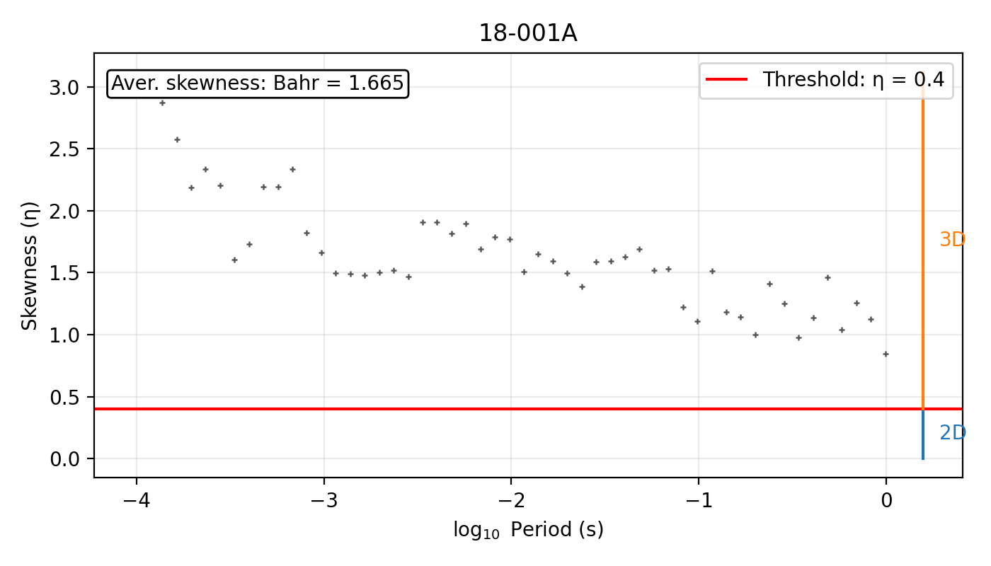
Every point for 18-001A sits above the red eta = 0.4 line,
consistent with the printed minimum of 0.85 above – the annotated
average, Bahr = 1.665, is itself more than four times the
threshold. Use this plot when you need to explain one station
concretely. Use the survey-wide phase-tensor plots below when the
question is line-scale dimensionality.
11.10.7. Masking By Skew#
mask_by_skew applies a phase-tensor skew threshold row by row. Every
mode reduces to the same shape – keep the row unless \(\beta\)
crosses a one-sided or two-sided bound – but which side of
\(\beta\) gets rejected changes with the mode:
Mode |
Keep rule |
Use it to |
|---|---|---|
|
\(|\beta| \le \text{thresh}\) |
reject rows too skewed in either direction – the usual symmetric threshold. |
|
\(\beta \le \text{thresh}\) |
reject only large positive skew, keeping large negative skew. |
|
\(\beta \ge \text{thresh}\) |
reject only large negative skew, keeping large positive skew. |
|
\(|\beta| \ge \text{thresh}\) |
the inverse of the default: keep only the strongly skewed rows, useful for isolating high-skew examples rather than removing them. |
"gt" and "lt" are asymmetric on purpose. They let a survey
tolerate skew of one sign – say, from a known distortion direction –
while still rejecting the other.
>>> from pycsamt.emtools import ensure_sites, mask_by_skew
>>> sites = ensure_sites("data/AMT/WILLY_DATA/L18PLT", recursive=True)
>>> masked = mask_by_skew(
...     sites,
...     thresh=6.0,
...     mode="abs_gt",
...     also="both",
...     inplace=False,
... )
>>> n_before = sum(int(getattr(s, "z").shape[0]) for s in sites)
>>> import numpy as np
>>> n_after = sum(int(np.isfinite(getattr(s, "z")).all(axis=(1, 2)).sum()) for s in masked)
>>> print(n_before, "rows total,", n_after, "rows survive |beta| <= 6")
1484 rows total, 397 rows survive |beta| <= 6
Barely more than a quarter of this survey’s rows clear a strict 6-degree threshold. That is a legitimate outcome for a genuinely high-skew line – not a sign the function misbehaved – and it is exactly why the next several sections build gentler alternatives to a flat row-by-row cutoff.
also controls which data blocks are masked:
"z"masks only impedance rows."tipper"masks only tipper rows."both"masks impedance and tipper rows at the same rejected frequencies.
The three non-default modes from the table above, in the same order:
>>> from pycsamt.emtools import mask_by_skew

>>> # Keep only rows with skew <= +6 degrees.
>>> keep_not_greater = mask_by_skew(sites, thresh=6.0, mode="gt")

>>> # Keep only rows with skew >= -6 degrees.
>>> keep_not_less = mask_by_skew(sites, thresh=-6.0, mode="lt")

>>> # Keep rows where absolute skew is at least 6 degrees.
>>> # This is unusual for inversion preparation, but useful for isolating
>>> # high-skew examples in diagnostics.
>>> keep_high_skew = mask_by_skew(sites, thresh=6.0, mode="abs_lt")
Because masking writes NaN into rejected tensor rows, always verify
how many usable rows remain before sending the result to an inversion or
plotting workflow.
11.10.8. Counting Surviving Rows#
A simple count helper is often enough for documentation and QC tables.
>>> import numpy as np
>>> from pycsamt.emtools import ensure_sites, mask_by_skew
>>> raw = ensure_sites("data/AMT/WILLY_DATA/L18PLT", recursive=True)
>>> masked = mask_by_skew(raw, thresh=6.0, also="z", inplace=False)
>>> rows = []
>>> for station in masked:
...     z = station.z
...     good = np.isfinite(z).all(axis=(1, 2))
...     rows.append(
...         {
...             "station": getattr(station, "name", ""),
...             "n_total": int(z.shape[0]),
...             "n_kept": int(good.sum()),
...             "kept_fraction": float(good.mean()),
...         }
...     )
...
>>> rows[:5]
[{'station': '18-001A', 'n_total': 53, 'n_kept': 28, 'kept_fraction': 0.5283018867924528}, {'station': '18-002U', 'n_total': 53, 'n_kept': 25, 'kept_fraction': 0.4716981132075472}, {'station': '18-003A', 'n_total': 53, 'n_kept': 19, 'kept_fraction': 0.3584905660377358}, {'station': '18-004A', 'n_total': 53, 'n_kept': 16, 'kept_fraction': 0.3018867924528302}, {'station': '18-005U', 'n_total': 53, 'n_kept': 18, 'kept_fraction': 0.33962264150943394}]
Even 18-001A, the lowest-median-skew station in the whole survey,
keeps barely over half its rows at this threshold. This count is the
sanity check that prevents a silent all-NaN result from moving
downstream. If strict thresholds keep too little data, return to the
skew distribution and decide whether a looser survey-specific threshold
is justified.
11.10.9. Longest Low-Skew Run#
keep_longest_low_skew is stricter than row-by-row masking. For each
station, it finds the longest contiguous frequency run satisfying
abs(skew) <= thresh and masks everything else.
>>> from pycsamt.emtools import ensure_sites, keep_longest_low_skew
>>> sites = ensure_sites("data/AMT/WILLY_DATA/L18PLT", recursive=True)
>>> banded = keep_longest_low_skew(
...     sites,
...     thresh=6.0,
...     min_len=3,
...     pad=1,
...     also="both",
...     fallback="keep_all",
...     inplace=False,
... )
>>> import numpy as np
>>> kept = [int(np.isfinite(s.z).all(axis=(1, 2)).sum()) for s in banded]
>>> print("kept rows per station (first 8):", kept[:8])
kept rows per station (first 8): [15, 14, 16, 13, 13, 9, 9, 10]
min_len is important. If a station has only one or two isolated
low-skew rows, you probably do not want to call that a usable band.
pad expands the selected run by a few neighboring frequencies.
The fallback controls what happens when no acceptable run exists:
fallback="keep_all"preserves the station rather than destroying it. This is safer for exploratory diagnostics, but it can make a failed threshold look like a fully accepted station unless you count rows.fallback="drop_all"masks the station completely when no run passes. This is stricter and should be used only when downstream code can handle missing stations or all-NaNrows.
11.10.10. Closing Small Gaps#
close_skew_gaps fills short interior gaps inside a low-skew mask.
It is useful when one or two noisy frequency samples break an otherwise
continuous band.
>>> import numpy as np
>>> from pycsamt.emtools import close_skew_gaps, ensure_sites, mask_by_skew
>>> sites = ensure_sites("data/AMT/WILLY_DATA/L18PLT", recursive=True)
>>> before = mask_by_skew(sites, thresh=6.0, mode="abs_gt", also="z", inplace=False)
>>> gap_closed = close_skew_gaps(
...     sites,
...     thresh=6.0,
...     max_gap=1,
...     also="both",
...     inplace=False,
... )
>>> n_before = sum(int(np.isfinite(s.z).all(axis=(1, 2)).sum()) for s in before)
>>> n_after = sum(int(np.isfinite(s.z).all(axis=(1, 2)).sum()) for s in gap_closed)
>>> print("rows kept before gap-closing:", n_before)
rows kept before gap-closing: 397
>>> print("rows kept after gap-closing:", n_after)
rows kept after gap-closing: 422
Bridging single-sample gaps recovers 25 more rows here, spread across
15 of the 28 stations – real frequencies that a strict row-by-row cut
had fragmented out of an otherwise continuous run. Set max_gap=0 to
disable gap closing. Increase it cautiously. A large value can bridge
unrelated good segments and create a band that no longer represents a
genuinely continuous low-skew interval.
11.10.11. Survey-Wide Low-Skew Band#
select_low_skew_band looks for frequencies supported by a fraction
of stations. It first builds each station’s own accepted band exactly as
keep_longest_low_skew would – the longest contiguous
\(|\beta| \le \text{thresh}\) run, extended by pad – and only
then projects every station’s band onto a shared union frequency grid
\(G\) and votes:
where \(N\) is the number of stations and \(\mathrm{band}_n\)
is station \(n\)’s own accepted run. A frequency survives only if
it falls inside the contiguous accepted band of at least a
frac-fraction of stations – not merely inside any low-skew row,
which is the weaker condition the vote-band plot below checks.
>>> from pycsamt.emtools import ensure_sites, select_low_skew_band
>>> sites = ensure_sites("data/AMT/WILLY_DATA/L18PLT", recursive=True)
>>> shared = select_low_skew_band(
...     sites,
...     thresh=6.0,
...     frac=0.6,
...     min_len=3,
...     pad=0,
...     also="both",
...     inplace=False,
... )
>>> import numpy as np
>>> kept = [int(np.isfinite(s.z).all(axis=(1, 2)).sum()) for s in shared]
>>> print("total kept:", sum(kept), "of", sum(int(s.z.shape[0]) for s in sites))
total kept: 0 of 1484
>>> shared_loose = select_low_skew_band(
...     sites,
...     thresh=12.0,
...     frac=0.4,
...     min_len=3,
...     pad=0,
...     also="both",
...     inplace=False,
... )
>>> kept_loose = [int(np.isfinite(s.z).all(axis=(1, 2)).sum()) for s in shared_loose]
>>> print("loosened (thresh=12, frac=0.4) total kept:", sum(kept_loose))
loosened (thresh=12, frac=0.4) total kept: 364
At the function’s own defaults, the survey-wide vote finds nothing:
the best-supported frequency has only 14 of 28 stations agreeing on
their own contiguous low-skew run, short of the 16.8 stations
frac=0.6 requires. That is a real, honest result for a line this
skewed, not a bug – it is exactly the “no clean shared window” finding
the traffic-light and ribbon plots below will confirm visually. Loosen
the criteria (here, thresh=12 and frac=0.4) and a genuine shared
band reappears, 364 rows this time. Use this function when you need one
common frequency band for a line, for example before a shared inversion
setup or a line-scale dimensionality statement; because it votes on
contiguous per-station bands rather than isolated pointwise passes, it
can legitimately return nothing even when individual stations and
periods look locally fine.
11.10.12. Traffic-Light Pseudo-Section#
plot_skew_traffic_psection colors each station-period cell by
absolute phase-tensor skew:
green:
abs(beta) <= t1;amber:
t1 < abs(beta) <= t2;red:
abs(beta) > t2.
>>> from pycsamt.emtools import ensure_sites, plot_skew_traffic_psection
>>> sites = ensure_sites("data/AMT/WILLY_DATA/L18PLT", recursive=True)
>>> fig, ax = plt.subplots(figsize=(10, 5))
>>> _ = plot_skew_traffic_psection(
...     sites,
...     t1=3.0,
...     t2=6.0,
...     axis_y="logperiod",
...     ax=ax,
... )
>>> fig.tight_layout()
>>> fig.savefig("skew_traffic_psection_l18plt.png", dpi=200)
>>> plt.close(fig)
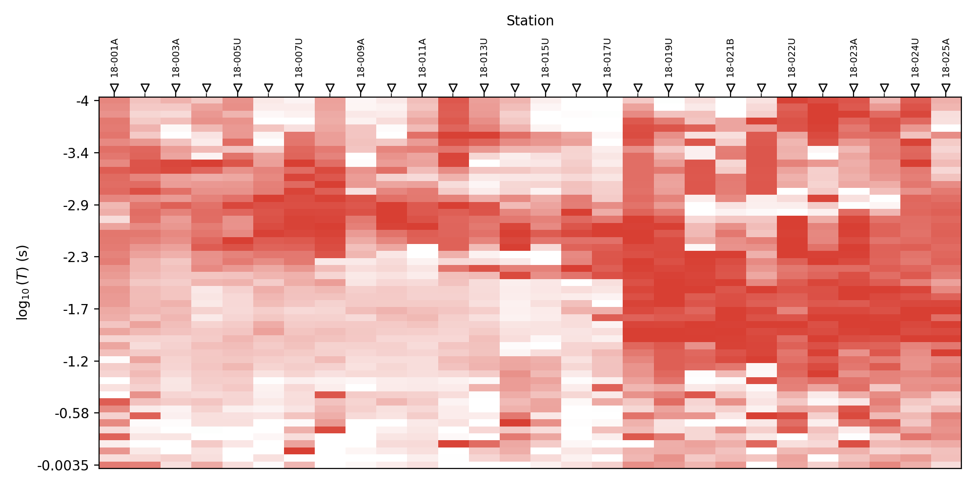
With strict t1=3/t2=6 thresholds, roughly 73 percent of this
survey’s cells read red, 12 percent amber, and 14 percent green –
visible here as a pseudo-section that is mostly pale red with only a
scattering of stronger colour, rather than solid red throughout. The
pattern is not random: the left half of the line (18-001A through
roughly 18-015U) is noticeably paler than the right half
(18-017U onward), the same early-versus-late split the station
summary table showed earlier. For highly skewed surveys like this one,
strict textbook thresholds are still useful – they tell you plainly
that a clean 2-D band does not exist without relaxing the criteria or
restricting to part of the line.
11.10.13. Percentile Ribbon#
plot_skew_percentile_ribbon summarizes the whole line by period. It
plots median absolute skew and percentile bands through the period axis.
>>> from pycsamt.emtools import ensure_sites, plot_skew_percentile_ribbon
>>> sites = ensure_sites("data/AMT/WILLY_DATA/L18PLT", recursive=True)
>>> fig, ax = plt.subplots(figsize=(8, 4))
>>> _ = plot_skew_percentile_ribbon(
...     sites,
...     n_bins=30,
...     q_lo=25.0,
...     q_hi=75.0,
...     extra=(10.0, 90.0),
...     ax=ax,
... )
>>> fig.tight_layout()
>>> fig.savefig("skew_percentile_ribbon_l18plt.png", dpi=200)
>>> plt.close(fig)
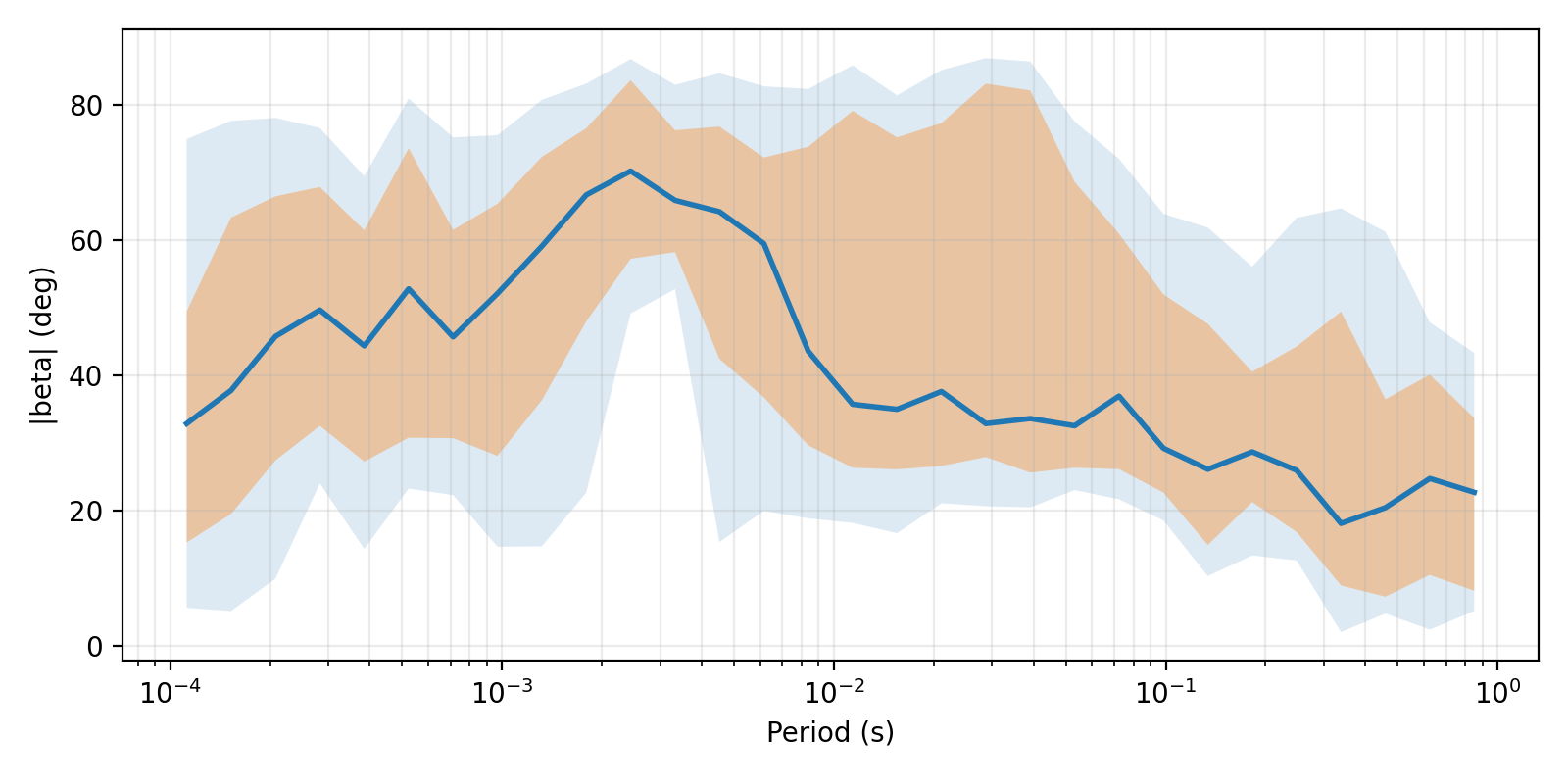
The median curve is genuinely period-dependent here: it stays under 15 degrees for periods shorter than about \(10^{-3}\,\mathrm{s}\), climbs into the 15-20 degree range through the middle of the band, and rises again toward 40-45 degrees at the longest periods – a real window rather than a uniformly high ribbon. Use this plot to answer: “Is there any period range where the line as a whole becomes less skewed?” Here, the answer is yes at short period, though even that window sits above a strict 3-6 degree threshold.
11.10.14. Vote-Band Plot#
plot_skew_vote_band bins the survey in log-period, and within each
bin \(b\) a station is counted as passing if a majority of its own
rows in that bin are low-skew:
where \(R_{n,b}\) is station \(n\)’s rows falling in bin
\(b\). This is a pointwise vote – it never checks whether a
station’s low-skew rows in neighboring bins are contiguous, which is
exactly what select_low_skew_band requires above. A period range can
therefore look well-supported here while still failing the stricter
survey-wide band selection.
>>> from pycsamt.emtools import ensure_sites, plot_skew_vote_band
>>> sites = ensure_sites("data/AMT/WILLY_DATA/L18PLT", recursive=True)
>>> fig, ax = plt.subplots(figsize=(8, 4))
>>> _ = plot_skew_vote_band(
...     sites,
...     thresh=6.0,
...     n_bins=40,
...     ax=ax,
... )
>>> fig.tight_layout()
>>> fig.savefig("skew_vote_band_l18plt.png", dpi=200)
>>> plt.close(fig)
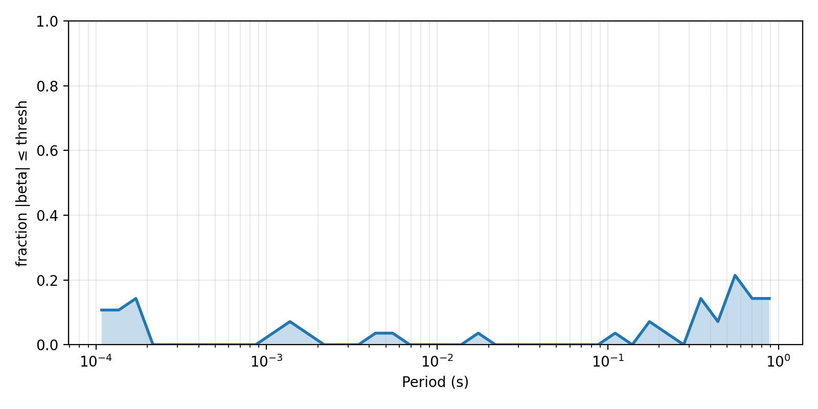
The vote fraction peaks near 0.9 at the very shortest periods, then
falls fast and spends most of the band oscillating under 0.4 – never
reaching the 0.6 support select_low_skew_band demanded by default
above. That is consistent with the empty result found there: plenty of
individual bins have some majority-passing stations, but not enough
overlap between which stations pass at which periods to satisfy a
stricter, contiguity-aware vote. Treat this plot as diagnostic rather
than a substitute for select_low_skew_band: a high vote here says
many stations are individually low-skew somewhere in the bin, not that
they share one continuous band.
11.10.15. Suggested Interpretation Pattern#
A robust skew review usually follows this sequence.
>>> from pycsamt.emtools import (
...     ensure_sites,
...     plot_skew_percentile_ribbon,
...     plot_skew_traffic_psection,
...     plot_skew_vote_band,
...     skew_table,
... )
>>> sites = ensure_sites("data/AMT/WILLY_DATA/L18PLT", recursive=True)
>>> table = skew_table(sites)
>>> table["skew"].abs().describe()
count    1484.000000
mean       23.850491
std        23.490731
min         0.050944
25%         5.375451
50%        14.920270
75%        37.654544
max        89.811834
Name: skew, dtype: float64
>>> fig, axes = plt.subplots(3, 1, figsize=(10, 12))
>>> _ = plot_skew_traffic_psection(sites, t1=3.0, t2=6.0, ax=axes[0])
>>> _ = plot_skew_percentile_ribbon(sites, ax=axes[1])
>>> _ = plot_skew_vote_band(sites, thresh=6.0, ax=axes[2])
>>> fig.tight_layout()
>>> fig.savefig("skew_review_panels_l18plt.png", dpi=200)
>>> plt.close(fig)
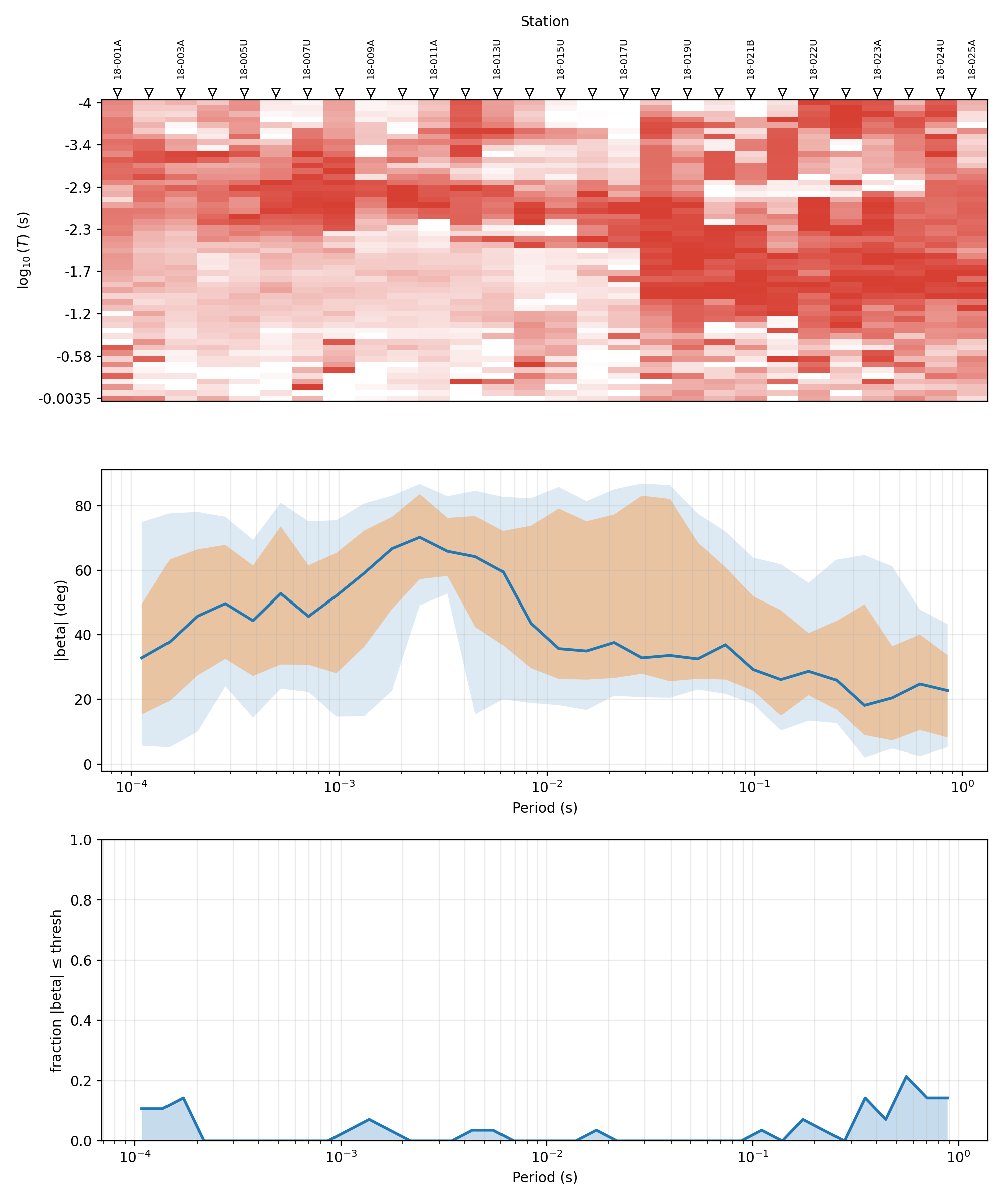
Read the three panels together, top to bottom: the pseudo-section
shows where on the line and at which periods skew is worst (the
right-hand, longer-period red block); the ribbon shows that the survey
median genuinely improves at short period rather than staying flat;
and the vote-band curve shows that even the best-supported period bins
fall well short of the majority needed for a shared band. Only after
reading all three together – not the summary table alone – should you
choose mask_by_skew, keep_longest_low_skew, close_skew_gaps,
or select_low_skew_band, and with which thresholds.
11.10.16. Pitfalls#
High skew is not automatically bad data. It may be the geologic signal. Use skew masks as interpretation tools, not as a reflexive cleaning step.
Do not compare Bahr \(\eta\) and phase-tensor \(\beta\) as if they have the same units. \(\eta\) is dimensionless; \(\beta\) is an angle in degrees.
Beware of fallback behavior in keep_longest_low_skew. If
fallback="keep_all", a station that fails the threshold completely
can return with all rows preserved. Count the surviving rows and inspect
the skew table.
Use also="z" when only impedance should drive downstream processing.
Use also="both" when tipper rows must stay aligned with impedance
masking.
11.10.17. Worked Example#
The example uses the L18PLT survey to compare phase-tensor skew and Bahr skewness, apply skew-based masks, keep contiguous low-skew bands, close small gaps, vote on a shared low-skew band, and generate the traffic-light, percentile-ribbon, vote-band, and Bahr-skew figures.
Open the rendered gallery page here: Phase-tensor and Bahr skew diagnostics (pycsamt.emtools.skew).