13.1. Site Containers#

The pycsamt.site.base module provides the station-centric containers used throughout the site layer. A container wraps either a EDI object or a modern EMTF XML document, without replacing either lower-level parser. Their purpose is to make common survey operations easier regardless of which format a station arrived in: station lookup, coordinate access, tensor inspection, DataFrame export, bulk selection, profile preparation, and writing cleaned sites back to disk.

The main objects are:

Object	Scope	Main use
`SiteMixin`	One EDI-like object site.	Shared accessors for name, coordinates, frequency, impedance, resistivity, phase, tipper, metadata, quality flags, and DataFrame export.
`Site`	One concrete station.	High-level wrapper around one `pycsamt.seg.edi.EDIFile` or one `EMTF` XML document, with a stable station identity and convenience edit helpers. See `Site.edi`, `Site.tf`, and `Site.backend`.
`Sites`	Many stations.	Ordered collection wrapper with integer indexing, name lookup, selection, batch edits, topography alignment, profile conversion, and export. Items may be a mix of EDI- and XML-backed `Site` objects.
`to_sites()`	API boundary helper.	Coerce compatible EDI- or EMTF-XML-like inputs (paths, objects, or mixed directories) into a `Sites` container.
`to_edis()`	API boundary helper.	Unwrap `Site` or `Sites` objects back to raw EDI objects or an `pycsamt.seg.collection.EDICollection`, materializing an EDI view for any XML-native site.

13.1.1. Where Containers Fit#

The site containers sit above pycsamt.seg and pycsamt.emtf, and below the higher-level workflow layers.

Layer	Main object	Responsibility
EDI parsing	`pycsamt.seg.edi.EDIFile`	Read, store, and write one EDI file.
EDI collection	`pycsamt.seg.collection.EDICollection`	Discover and parse many EDI files from paths, folders, or glob patterns.
EMTF-XML document	`pycsamt.emtf.document.EMTF`	Read, hold, and write one format-neutral transfer function, with the full Metadata object tree. See EMTF.
Site layer	`Site`, `Sites`	Expose station-oriented accessors, editing, filtering, summaries, and survey preparation helpers, transparently over either format.
Downstream workflows	Selection, diagnostics, export, profiles, inversion, agents.	Use prepared site containers as consistent inputs.

Use EDIFile/EDICollection or EMTF directly when you are primarily parsing one format and need its own low-level API (see EMTF for the latter). Use Site or Sites when you are preparing, inspecting, selecting, or editing station data.

13.1.2. Creating One Site#

Create a Site from a parsed pycsamt.seg.edi.EDIFile. The examples on this page use one line of the bundled WILLY AMT survey, data/AMT/WILLY_DATA/L18PLT, so every printed value below is real output from real stations rather than a sketch.

>>> from pycsamt.seg.edi import EDIFile
>>> from pycsamt.site.base import Site

>>> edi = EDIFile("data/AMT/WILLY_DATA/L18PLT/18-001A.edi")
>>> site = Site(edi)

>>> print(site.name)
>>> print(site.coords)
>>> print(site.summary())
18-001A
(32.1203, 119.12883333333333, 99.0)
{'name': '18-001A', 'nfreq': 53, 'lat': 32.1203, 'lon': 119.12883333333333,
 'elev': 99.0, 'components': ['Zxx', 'Zxy', 'Zyx', 'Zyy'], 'tipper': False}

The wrapper keeps the original EDI object available as site.edi and through Site.to_edi(). Prefer the Site accessors for routine work, and unwrap to EDI only when you need lower-level EDI functionality.

>>> raw = site.to_edi()
>>> detached = site.to_edi(copy=True)

13.1.3. Station Identity#

Station identity is normalized from EDI HEAD fields. The name resolution order is:

dataid;
station;
sitename;
name;
STATION;
the file stem, when header fields are missing.

When a Site is created, the constructor attempts to stabilize the EDI header so that dataid and, when absent, station match the resolved site stem. This makes name lookup and downstream joins more predictable.

>>> site = Site(EDIFile("data/AMT/WILLY_DATA/L18PLT/18-012A.edi"))

>>> print(site.name)
18-012A
>>> print(site.meta)
{'station': '18-012A', 'lat': 32.13016666666667, 'lon': 119.12876666666666,
 'elev': 126.0, 'dataid': '18-012A'}

Here dataid already agreed with the file stem, so stabilization left it untouched; on a file where the header disagreed with the stem, this same step is what keeps site.name predictable. Rename a site with Site.rename():

>>> renamed = site.rename("L01_012")

>>> print(site.name)      # original unchanged
18-012A
>>> print(renamed.name)   # new wrapper
L01_012

Use inplace=True when the existing wrapper should be modified:

>>> site.rename("L01_012", inplace=True)

13.1.4. Coordinates#

Coordinates are exposed as (lat, lon, elev) in decimal degrees and meters. Continuing with the renamed site from the previous section:

>>> lat, lon, elev = site.coords
>>> print(lat, lon, elev)
32.13016666666667 119.12876666666666 126.0

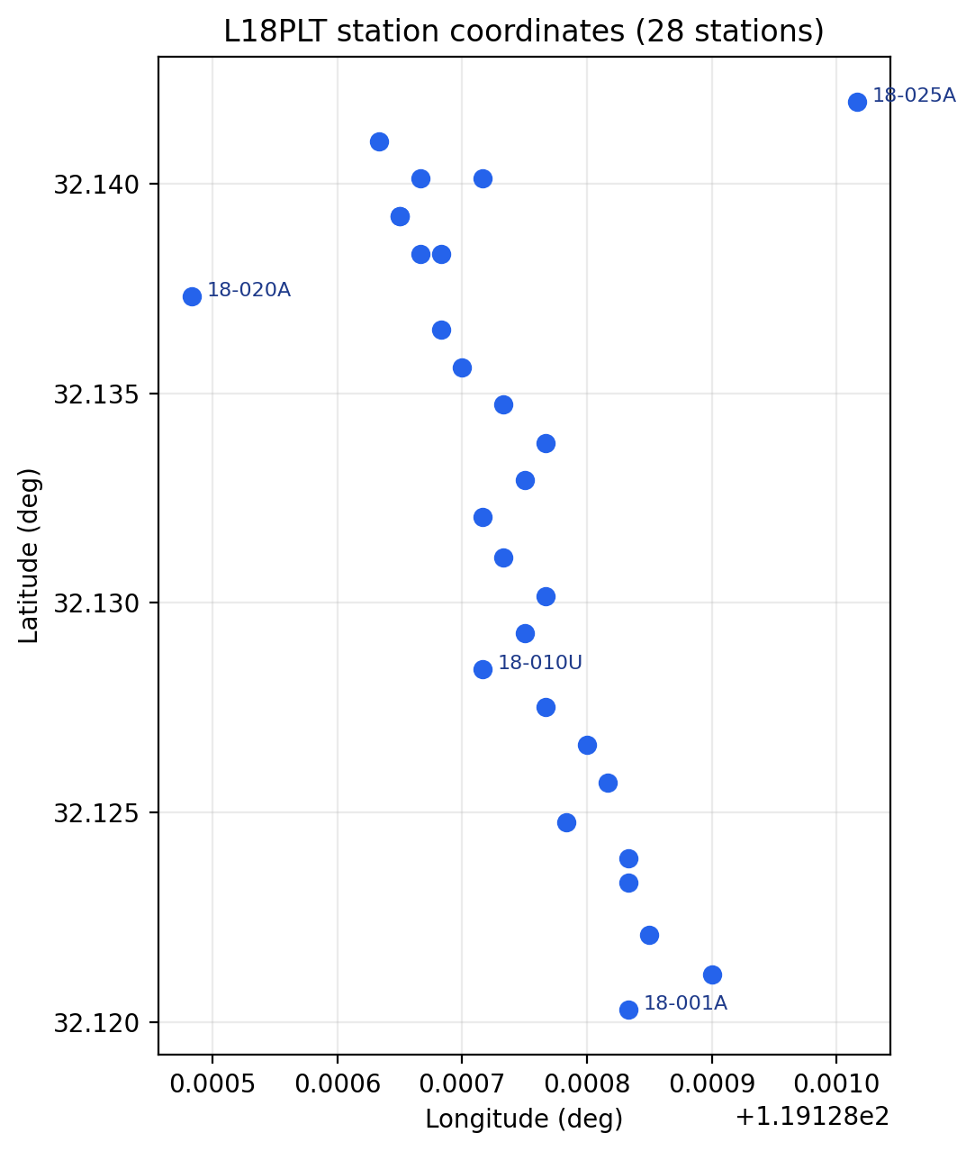
../../_images/user-guide-site-containers-01.png — The 28 stations of the `L18PLT` line plotted from `site.coords`. Real field lines are rarely perfectly straight; `18-020A` sits off to one side, which is exactly the kind of thing a quick coordinate scatter catches before it surprises a profile or map view later.#

Update coordinates with Site.set_coords():

>>> moved = site.set_coords(10.25, 20.75, 640.0)
>>> print(moved.coords)
(10.25, 20.75, 640.0)

Like Site.rename(), coordinate updates are copy-returning by default and in-place when requested:

>>> site.set_coords(10.25, 20.75, 640.0, inplace=True)

13.1.5. Array Accessors#

The container exposes the most common station arrays as properties.

At each angular frequency \(\omega=2\pi f\), the horizontal electric and magnetic field phasors are related by the complex impedance tensor

(1)#\[\begin{split}\begin{bmatrix}E_x\\E_y\end{bmatrix} = \begin{bmatrix}Z_{xx} & Z_{xy}\\Z_{yx} & Z_{yy}\end{bmatrix} \begin{bmatrix}H_x\\H_y\end{bmatrix}.\end{split}\]

Thus site.z[k, i, j] is \(Z_{ij}\) at site.freq[k]. The rho and phase arrays are not independent observations: for each component they are derived from the same complex value as

(2)#\[\rho_{a,ij}(f)=\frac{|Z_{ij}(f)|^2}{\mu_0\,2\pi f}, \qquad \phi_{ij}(f)=\operatorname{atan2} \!\left(\Im Z_{ij},\Re Z_{ij}\right)\frac{180}{\pi},\]

when impedance is expressed in SI units. EDI field units use the equivalent conversion factor during parsing. Equations (1) and (2) explain why frequency, impedance, resistivity, and phase must retain the same first-axis ordering.

Property	Meaning	Shape convention
`freq`	Frequency grid in Hz.	`(n_freq,)`.
`z`	Complex impedance tensor.	Usually `(n_freq, 2, 2)`; flattened internally as `Zxx, Zxy, Zyx, Zyy` when exported.
`z_err`	Impedance uncertainty.	Aligned with `z` when present.
`rho`	Apparent resistivity.	Aligned with impedance components.
`phase`	Impedance phase in degrees.	Aligned with impedance components.
`tipper`	Vertical magnetic transfer function (tipper).	`(n_freq, 2)` with `Tx` and `Ty`.
`meta`	Header and optional `INFO` metadata.	Python dictionary.

Example:

>>> print(site.freq)
>>> print(site.z.shape if site.z is not None else "no Z")
>>> print(site.quality_flags())
[1.040e+04 8.707e+03 7.289e+03 6.102e+03 5.108e+03 4.277e+03 3.580e+03
 2.997e+03 2.509e+03 2.101e+03 1.759e+03 1.472e+03 1.233e+03 1.032e+03
 8.639e+02 7.232e+02 6.054e+02 5.069e+02 4.243e+02 3.552e+02 2.974e+02
 2.490e+02 2.084e+02 1.745e+02 1.461e+02 1.223e+02 1.024e+02 8.571e+01
 7.175e+01 6.007e+01 5.029e+01 4.210e+01 3.525e+01 2.951e+01 2.470e+01
 2.068e+01 1.731e+01 1.449e+01 1.213e+01 1.016e+01 8.504e+00 7.119e+00
 5.960e+00 4.990e+00 4.177e+00 3.497e+00 2.928e+00 2.451e+00 2.052e+00
 1.718e+00 1.438e+00 1.204e+00 1.008e+00]
(53, 2, 2)
{'has_freq': True, 'has_z': True, 'has_z_err': True, 'has_rho': True,
 'has_phase': True, 'has_tipper': False}

This station carries the full 53-frequency AMT band and a complete impedance tensor, but no tipper – has_tipper is False rather than missing or raising, which is what lets the next section branch on it safely.

13.1.6. Quality And Component Checks#

Use Site.quality_flags() for coarse array availability checks.

>>> flags = site.quality_flags()
>>> print(flags)

>>> if not flags["has_z"]:
...     print(f"{site.name} has no finite impedance tensor")
{'has_freq': True, 'has_z': True, 'has_z_err': True, 'has_rho': True,
 'has_phase': True, 'has_tipper': False}

Nothing is printed by the if branch here, because has_z is True for this station; the branch only fires for a station whose impedance tensor is missing or non-finite. Use Site.has_component() when a specific impedance or tipper component matters.

>>> if site.has_component("Zxy") and site.has_component("Zyx"):
...     print("off-diagonal impedance components are available")
...
>>> if site.has_component("tipper"):
...     print("tipper is available")
off-diagonal impedance components are available

The second if prints nothing, consistent with has_tipper being False above – has_component("tipper") and quality_flags() agree because they read the same underlying arrays. Supported impedance component names are Zxx, Zxy, Zyx, and Zyy: the diagonal pair and the off-diagonal components Zxy/Zyx checked just above. Tipper checks accept tip, tx, ty, and tipper.

13.1.7. DataFrame Export#

Site.to_dataframe() exports core arrays into frequency-indexed pandas.DataFrame objects. This is the quickest way to inspect one station in a notebook or build masks for editing.

>>> z = site.to_dataframe("z")
>>> rp = site.to_dataframe("resphase")
>>> tip = site.to_dataframe("tipper")

>>> print(z.head())
>>> print(rp.head())
>>> print(tip.head())
                  Zxx             Zxy             Zyx           Zyy
f
10400.0  51.63+94.43j  1737.0+ 922.4j -2235.0- 754.6j -132.7+278.8j
8707.0   40.43+70.87j  1681.0+ 929.9j -2176.0- 745.4j -177.3+287.3j
7289.0   21.00+34.14j  1558.0+ 938.8j -2102.0- 773.9j -239.8+253.6j
6102.0   47.11+16.06j  1383.0+ 922.5j -2032.0- 783.7j -237.9+180.2j
5108.0   61.44-90.83j  1261.0+ 844.8j -1776.0- 602.6j -130.9+263.3j

          rho_zxx    phi_zxx    rho_zxy  ...     phi_zyx   rho_zyy     phi_zyy
f                                        ...
10400.0  0.222744  61.332181  74.384438  ... -161.343845  1.833437  115.452974
8707.0   0.152915  60.296056  84.770300  ... -161.090840  2.618045  121.679771
7289.0   0.044081  58.403736  90.786375  ... -159.787647  3.342489  133.397901
6102.0   0.081196  18.824462  90.583260  ... -158.909414  2.919320  142.857487
5108.0   0.470829 -55.924459  90.203917  ... -161.257833  3.385345  116.434339

[5 rows x 8 columns]
Empty DataFrame
Columns: []
Index: [10400.0, 8707.0, 7289.0, 6102.0, 5108.0]

tip comes back with no columns at all: this station has no tipper, so to_dataframe("tipper") returns an empty frame that still carries the correct frequency index rather than raising. Note rho_zxx here is small and phi_zxx swings from positive to negative between rows – the diagonal components are far noisier than the off-diagonal rho_zxy/rho_zyx pair, which is typical and part of why interpretation usually leans on the off-diagonal components first. The accepted kind values are:

Kind	Aliases	Columns
`"z"`	`"imp"`, `"impedance"`	`Zxx`, `Zxy`, `Zyx`, `Zyy`.
`"resphase"`	`"rp"`, `"rho_phase"`	`rho_zxx`, `phi_zxx`, `rho_zxy`, `phi_zxy`, and the equivalent `Zyx`/`Zyy` columns.
`"tipper"`	`"tip"`, `"t"`	`Tx`, `Ty`.

Pass api=True when a pyCSAMT APIFrame is required:

>>> frame = site.to_dataframe("z", api=True)
>>> print(frame.kind)
>>> print(frame.df.head())
site.z
                  Zxx             Zxy             Zyx           Zyy
f
10400.0  51.63+94.43j  1737.0+ 922.4j -2235.0- 754.6j -132.7+278.8j
8707.0   40.43+70.87j  1681.0+ 929.9j -2176.0- 745.4j -177.3+287.3j
7289.0   21.00+34.14j  1558.0+ 938.8j -2102.0- 773.9j -239.8+253.6j
6102.0   47.11+16.06j  1383.0+ 922.5j -2032.0- 783.7j -237.9+180.2j
5108.0   61.44-90.83j  1261.0+ 844.8j -1776.0- 602.6j -130.9+263.3j

frame.kind is a stable tag ("site.z") rather than a class name, so code that branches on it does not need to import Site just to recognize what a frame holds.

13.1.8. Creating A Collection#

Use Sites when working with more than one station.

>>> from pycsamt.seg.edi import EDIFile
>>> from pycsamt.site.base import Sites

>>> edis = [
...     EDIFile("data/AMT/WILLY_DATA/L18PLT/18-001A.edi"),
...     EDIFile("data/AMT/WILLY_DATA/L18PLT/18-002U.edi"),
...     EDIFile("data/AMT/WILLY_DATA/L18PLT/18-003A.edi"),
... ]

>>> sites = Sites(edis)

>>> print(len(sites))
>>> print([site.name for site in sites])
3
['18-001A', '18-002U', '18-003A']

If your input is a directory or glob pattern, parse it first with pycsamt.seg.collection.EDICollection, then wrap it:

>>> from pycsamt.seg.collection import EDICollection
>>> from pycsamt.site.base import Sites

>>> collection = EDICollection.from_sources("data/AMT/WILLY_DATA/L18PLT")
>>> sites = Sites(collection)

>>> print(len(sites))
28

That is the whole L18PLT line rather than the three-station subset above – sites is reassigned here, and the rest of this page continues from this 28-station collection. For API boundaries that may receive several input types, use to_sites():

>>> from pycsamt.site.base import to_sites

>>> sites = to_sites(collection)
>>> print(len(sites))
28

13.1.9. Working With EMTF-XML#

Every example so far has built a Site from an EDIFile. Site accepts an EMTF XML document exactly the same way, via Site.from_xml(). The examples below use the real Gabbs Valley station gv100 (public-domain USGS data, doi:10.5066/P9GZ9Z56), bundled both as EDI (data/gv_data/gv_final_edi/gv100.edi) and as the EMTF-XML pyCSAMT converted it to (data/gv_data/xml/gv100.xml) – the same file already used throughout Metadata and EMTF.

>>> from pycsamt.site.base import Site

>>> xml_site = Site.from_xml("data/gv_data/xml/gv100.xml")

>>> print(xml_site.backend)
>>> print(xml_site.name)
>>> print(xml_site.coords)
xml
gv100
(38.6113805555556, -118.535261111111, 1437.4)

Site.backend reports which format is native – informational only, since every SiteMixin accessor used earlier on this page (name, coords, freq, z, rho, phase, tipper, to_dataframe(), quality_flags(), has_component(), summary()) works identically regardless of it. Loading the matching EDI file confirms the two representations agree numerically:

>>> edi_site = Site.from_edi("data/gv_data/gv_final_edi/gv100.edi")

>>> import numpy as np
>>> print(np.allclose(edi_site.z, xml_site.z))
True

13.1.9.1. Lazy Materialization#

Site.edi and Site.tf are both always available on any Site, regardless of which one it was built from. The representation not natively supplied is materialized from the other on first access, via pycsamt.emtf.converters.edi.edi_to_emtf()/emtf_to_edi (see EDI Interoperability), and cached – so xml_site.z above already triggered a real EDI materialization behind the scenes the first time it ran. The effect is visible on Site.meta, which reads directly from the XML document when nothing has forced materialization yet, but falls back to the plain EDI-header dictionary once it has:

>>> fresh = Site.from_xml("data/gv_data/xml/gv100.xml")
>>> print(fresh.meta)
{'station': 'gv100', 'dataid': 'gv100', 'name': 'Gabbs Valley',
 'sitename': 'Gabbs Valley', 'lat': 38.6113805555556,
 'lon': -118.535261111111, 'elev': 1437.4}

>>> print(fresh.z.shape)          # forces materialization
(48, 2, 2)

>>> print(fresh.meta)             # now the plain EDI-header view
{'lat': 38.6113805555556, 'lon': -118.535261111111, 'elev': 1437.4,
 'dataid': 'gv100'}

Neither dictionary is wrong – meta has always been the lean, EDI-shaped summary documented in “Array Accessors” above. The richer view, available whenever a Site is (or still is) XML-native, comes from a set of typed properties that return the same pycsamt.metadata objects the EMTF document itself holds, not a copy:

>>> rich = Site.from_xml("data/gv_data/xml/gv100.xml")
>>> print(rich.site_meta.name, "/", rich.site_meta.survey)
>>> print(rich.provenance.creator.name)
Gabbs Valley / GV2020
Jared Peacock

Site.site_meta, Site.site_layout, Site.provenance, Site.processing, Site.copyright, and Site.quality_meta mirror EMTF’s own attributes exactly. See Metadata for what each object holds and EMTF for how they round-trip through EDI and XML.

13.1.9.2. Writing And Discovering XML#

Site.to_xml() writes a document back out; without a target it returns the XML as a string:

>>> text = edi_site.to_xml()
>>> print(text.splitlines()[:2])
['<?xml version="1.0" encoding="UTF-8"?>', '<EM_TF>']

Sites accepts a mix of EDI- and XML-backed stations directly:

>>> from pycsamt.site.base import Sites

>>> mixed = Sites([edi_site, xml_site])
>>> print(len(mixed))
>>> print([s.backend for s in mixed])
2
['edi', 'xml']

and to_sites() – the same coercion ensure_sites() uses – discovers a directory of *.xml files (or a directory mixing *.edi and *.xml) the same way it already discovers EDI directories:

>>> from pycsamt.site.base import to_sites

>>> discovered = to_sites("data/gv_data/xml")
>>> print(len(discovered))
>>> print(sorted(s.name for s in discovered))
3
['gv100', 'gv101', 'gv102']

Sites.write_xml() and Sites.to_emtf_list() are the XML-side counterparts of Sites.write() and Sites.to_edis():

>>> paths = discovered.write_xml("outputs/clean_xml")
>>> for path in paths:
...     print(path)
outputs/clean_xml/gv100.xml
outputs/clean_xml/gv101.xml
outputs/clean_xml/gv102.xml

13.1.10. Unwrapping Back To EDI#

The site layer is intentionally reversible. Use to_edis() when a workflow has prepared, filtered, renamed, or edited Site objects but the next function expects raw EDI objects.

>>> from pycsamt.site.base import to_edis

>>> raw = to_edis(site)
>>> edis = to_edis(sites)
>>> collection = to_edis(sites, as_collection=True)

>>> print(type(raw).__name__)
>>> print(len(edis))
>>> print(type(collection).__name__, len(collection))
EDIFile
28
EDICollection 28

Here site is the single L01_012 wrapper from the top of this page, so raw is one EDIFile; sites is the 28-station collection, so edis is a plain list and collection is an EDICollection of the same length. By default, unwrapping is shallow: the returned EDI objects are the same objects stored by the wrappers. Pass copy=True when the caller should be able to mutate the returned objects independently.

>>> detached_edis = to_edis(sites, copy=True)
>>> print(len(detached_edis))
28

The helper also accepts mixed inputs, path-like sources, raw EDI objects, and existing EDICollection instances. Invalid items are skipped unless strict=True is requested.

>>> edis = to_edis([site, raw, "data/AMT/WILLY_DATA/L18PLT"], strict=False)
>>> print(len(edis))

>>> checked = to_edis(sites, strict=True, progress=True)
>>> print(len(checked))
29
28

site and raw both point at the same underlying L01_012 EDI object – raw was produced by site.to_edi() above, so it is not a second station – and the directory contributes the other 28, for 29 total rather than 30. progress=True draws a text progress bar while unwrapping; it does not change checked itself, which is still the 28-station list. Use the collection methods when you are already holding a Sites instance:

>>> edis = sites.to_edis()
>>> collection = sites.to_edicollection(copy=True)

>>> print(len(edis))
>>> print(type(collection).__name__, len(collection))
28
EDICollection 28

Sites.from_any is another entry point when you want pyCSAMT’s session normalization to interpret heterogeneous inputs:

>>> sites = Sites.from_any("data/AMT/WILLY_DATA/L18PLT")
>>> print(len(sites))
28

13.1.11. Collection Lookup#

Sites preserves input order and supports integer indexing, case-insensitive name lookup, and safe lookup.

>>> first = sites[0]
>>> same = sites.by_index(0)
>>> station = sites["18-002u"]
>>> maybe = sites.get("missing")

>>> print(first.name)
>>> print(same.name)
>>> print(station.name)
>>> print(maybe is None)
18-001A
18-001A
18-002U
True

The lookup "18-002u" finds 18-002U regardless of case, which is the same case-insensitive matching Site.rename() and Sites.select() rely on for station identity. sites["missing"] raises KeyError. Use Sites.get() when missing stations are acceptable.

The Sites.as_list() method returns the underlying EDI objects:

>>> edi_objects = sites.as_list()
>>> print(len(edi_objects), type(edi_objects[0]).__name__)
28 EDIFile

This is useful when passing a prepared collection into utilities that still operate directly on EDI objects. For new API boundaries, prefer Sites.to_edis() or to_edis() because they also support copying, progress display, strict validation, and collection output.

13.1.12. Mapping And Selection#

Use Sites.map() to apply a lightweight operation to every station:

>>> names = sites.map(lambda site: site.name)
>>> coverage = sites.map(lambda site: site.summary()["nfreq"])

>>> print(names)
>>> print(coverage[:8], "...")
['18-001A', '18-002U', '18-003A', '18-004A', '18-005U', '18-006A',
 '18-007U', '18-008U', '18-009A', '18-010U', '18-011A', '18-012A',
 '18-013U', '18-014A', '18-015U', '18-016A', '18-017U', '18-018A',
 '18-019U', '18-020A', '18-021B', '18-021U', '18-022U', '18-022V',
 '18-023A', '18-023V', '18-024U', '18-025A']
[53, 53, 53, 53, 53, 53, 53, 53] ...

Every station on this line shares the same 53-row frequency grid, so coverage is a flat list of 53s here; on a mixed survey this is the first place a shorter frequency run would show up. For simple collection filtering, use Sites.select():

>>> subset = sites.select(names=["18-001A", "18-003A"])
>>> with_zxy = sites.select(predicate=lambda site: site.has_component("Zxy"))

>>> print(len(subset), [s.name for s in subset])
>>> print(len(with_zxy))
2 ['18-001A', '18-003A']
28

All 28 stations keep an off-diagonal Zxy component here, so with_zxy comes back the same size as sites; on noisier data this is a quick way to see how many stations would survive a component requirement. For richer selection by glob names, frequency coverage, coordinates, chainage, or data quality, use the functions documented in Site Selection.

13.1.13. Bulk Edits#

Sites.edit_all() applies common operations across the collection.

>>> renamed = sites.edit_all(
...     rename=lambda name: f"LINE01_{name}",
...     inplace=False,
... )

>>> sliced = sites.edit_all(
...     freq_slice=slice(1, None),
...     inplace=False,
... )

>>> print([s.name for s in renamed][:5])
>>> print(len(sliced[0].freq), len(sites[0].freq))
['LINE01_18-001A', 'LINE01_18-002U', 'LINE01_18-003A', 'LINE01_18-004A',
 'LINE01_18-005U']
52 53

freq_slice=slice(1, None) drops the first (highest) frequency from every station, so each sliced site carries 52 rows against 53 on the untouched sites. The optional mask callback receives the output of site.to_dataframe("z") and returns a boolean mask. Rows where the mask is False are set to NaN in the impedance tensor.

>>> def keep_lower_frequencies(frame):
...     cutoff = frame.index.to_series().median()
...     return frame.index <= cutoff
...
>>> masked = sites.edit_all(mask=keep_lower_frequencies)
>>> print(masked[0].to_dataframe("z").notna().sum())
Zxx    27
Zxy    27
Zyx    27
Zyy    27
dtype: int64

Half of the 53 rows survive the median cutoff, as expected for a mask built from the frame’s own median. Use pycsamt.site.edit when you need more explicit editing functions such as tensor rotation, coordinate table assignment, frequency range selection, or resistivity/phase recomputation.

13.1.14. Topography Alignment#

Sites.with_topography() updates site coordinates and elevation from a table-like object. Station identifiers are matched by normalized names.

>>> import pandas as pd

>>> print(sites["18-001A"].coords)
>>> print(sites["18-002U"].coords)

>>> topo = pd.DataFrame(
...     {
...         "station": ["18-001A", "18-002U"],
...         "latitude": [32.1205, 32.1212],
...         "longitude": [119.12890, 119.12895],
...         "elevation": [101.5, 112.0],
...     }
... )

>>> updated = sites.with_topography(topo, inplace=False)
>>> print(updated["18-001A"].coords)
>>> print(updated["18-002U"].coords)
(32.1203, 119.12883333333333, 99.0)
(32.12113333333333, 119.12889999999999, 110.0)
(32.1205, 119.1289, 101.5)
(32.1212, 119.12895, 112.0)

Only the two named stations moved; the other 26 stations in sites keep their original EDI-header coordinates because unmatched stations are left unchanged. Use this after loading raw EDI files when field GPS or corrected elevation tables are authoritative.

13.1.15. Closest Site#

Sites.closest() finds the nearest station to a target coordinate using geodetic distance, which is what makes it meaningful to search by plain latitude/longitude rather than a projected offset.

For coordinates in radians, the distance tested against tol is the haversine distance

(3)#\[d=2R\arcsin\!\sqrt{ \sin^2\!\left(\frac{\phi_2-\phi_1}{2}\right) +\cos\phi_1\cos\phi_2 \sin^2\!\left(\frac{\lambda_2-\lambda_1}{2}\right)},\]

where \(R\) is Earth radius, \(\phi\) is latitude, and \(\lambda\) is longitude. This makes the 50 m tolerance below a physical surface distance rather than a difference in decimal degrees.

>>> target_lat, target_lon = 32.1211, 119.12888
>>> nearest = sites.closest(lat=target_lat, lon=target_lon)

>>> if nearest is not None:
...     print(nearest.name)
18-002U

The target here is a stand-in for a field GPS fix a few metres from 18-002U’s header coordinate; closest resolves it to that station without needing an exact match. Add tol in meters when a maximum distance is required:

>>> nearest = sites.closest(lat=target_lat, lon=target_lon, tol=50.0)
>>> print(nearest.name if nearest is not None else None)

>>> too_strict = sites.closest(lat=target_lat, lon=target_lon, tol=1.0)
>>> print(too_strict)
18-002U
None

If the closest station is farther than tol, the method returns None – here a 1-metre tolerance is tighter than the actual offset, so the second call comes back empty even though a station clearly exists nearby.

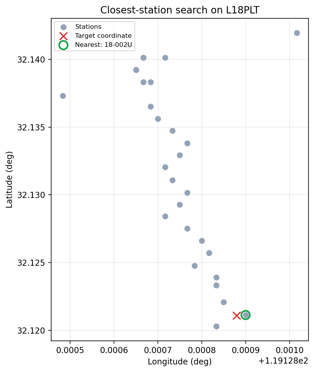
../../_images/user-guide-site-containers-02.png — Target coordinate (red cross) resolved to the nearest station (green ring) among the 28 stations of `L18PLT`.#

13.1.16. Profiles#

Sites.to_profile() converts station coordinates into a survey-line profile for line-ordered work, sorting stations by chainage rather than by name. An origin and azimuth define the line; a natural choice is the first station and the geodetic distance bearing toward the last one:

>>> from pycsamt.site.location import bearing

>>> first_s = sites[0]
>>> last_s = sites.by_index(len(sites) - 1)
>>> azimuth = bearing(first_s.coords[:2], last_s.coords[:2])
>>> print(round(azimuth, 3))
0.411

An azimuth near zero confirms L18PLT runs almost due north, which is consistent with the mostly-vertical scatter in the coordinate plot above.

>>> origin = (first_s.coords[0], first_s.coords[1])
>>> profile = sites.to_profile(origin=origin, azimuth=azimuth)

>>> if hasattr(profile, "chainages"):
...     for name, chainage in sorted(
...         profile.chainages.items(), key=lambda kv: kv[1]
...     )[:6]:
...         print(name, round(chainage, 2))
>>> else:
...     print([site.name for site in profile["sites"]])
18-001A 0.0
18-002U 92.54
18-003A 197.96
18-004A 336.69
18-005U 399.59
18-006A 495.75

18-001A sits at the origin by construction, so its chainage is 0.0; each later station’s chainage is its signed distance along azimuth from that origin. In local east–north offsets \((\Delta e,\Delta n)\), the projection used to order the line is

(4)#\[s=\Delta e\sin A+\Delta n\cos A,\]

with azimuth \(A\) measured clockwise from north. Positive values in the transcript therefore lie forward from the origin along the inferred line; an off-line displacement contributes only its projection onto that direction. When pycsamt.site.profile.Profile is available, the method returns a rich profile object exposing chainages as a {station: metres} dictionary, as above. Otherwise it returns a fallback dictionary containing origin, azimuth, and line-ordered sites.

For more control over profile inference, chainage, and spacing statistics, continue to Location And Profiles.

13.1.17. Writing Sites#

Sites.write() writes one EDI file per station into a directory.

>>> paths = sites.write(
...     "outputs/clean_edi",
...     template="{station}.edi",
...     exist_ok=True,
... )

>>> for path in paths:
...     print(path)
outputs/clean_edi/18-001A.edi
outputs/clean_edi/18-002U.edi
outputs/clean_edi/18-003A.edi
outputs/clean_edi/18-004A.edi
outputs/clean_edi/18-005U.edi
...
28 files written

Use Sites.write_xml() instead for the EMTF-XML equivalent (see “Working With EMTF-XML” above). For richer export workflows, including manifest CSV files and zip packages, use the functions documented in Export And Reporting.

13.1.18. Common Patterns#

Inspect one station:

>>> site = sites["18-001A"]
>>> print(site.summary())
>>> print(site.to_dataframe("resphase").head())
{'name': '18-001A', 'nfreq': 53, 'lat': 32.1203, 'lon': 119.12883333333333,
 'elev': 99.0, 'components': ['Zxx', 'Zxy', 'Zyx', 'Zyy'], 'tipper': False}

Build a QC table:

>>> import pandas as pd

>>> qc = pd.DataFrame([site.summary() for site in sites])
>>> print(qc[["name", "nfreq", "components", "tipper"]])
      name  nfreq            components  tipper
0  18-001A     53  [Zxx, Zxy, Zyx, Zyy]   False
1  18-002U     53  [Zxx, Zxy, Zyx, Zyy]   False
2  18-003A     53  [Zxx, Zxy, Zyx, Zyy]   False
...
27  18-025A     53  [Zxx, Zxy, Zyx, Zyy]   False

[28 rows x 4 columns]

A QC table like this is the fastest way to spot a station that fell short of the survey’s frequency count or is missing a component, before it reaches plotting or inversion. Select, align, and export:

>>> selected = sites.select(predicate=lambda site: site.has_component("Zxy"))
>>> updated = selected.with_topography(topo)
>>> updated.write("outputs/selected_edi", exist_ok=True)

13.1.19. Common Mistakes#

Assuming every object has Sites.from_path: Use pycsamt.seg.collection.EDICollection.from_sources, Sites.from_any(), or to_sites() depending on the input form.
Editing site.edi directly during routine workflows: Direct EDI edits are sometimes necessary, but the site helpers keep name, coordinate, and array conventions more consistent.
Forgetting copy versus in-place behaviour: Site.rename(), Site.set_coords(), Site.set_empty(), Sites.edit_all(), and Sites.with_topography() return new objects by default unless inplace=True is used.
Comparing station names before normalization: Wrap EDI files as Site or Sites before doing name-based joins or lookups, so comparisons see the same resolved station identity on both sides.
Using summary as a substitute for data inspection: summary is a quick overview. Use Site.to_dataframe(), Site.quality_flags(), and the diagnostics in Computed Diagnostics for deeper checks.
Assuming Site is EDI-only: Site and Sites accept EMTF XML documents and directories of *.xml files too – see “Working With EMTF-XML” above. Code written against site.z/site.freq/etc. does not need to change to support both.

13.1.20. Next Pages#

Continue with:

Site Selection for station filtering;
Site Editing for explicit single-site and collection edits;
Location And Profiles for coordinates, topography, distances, and chainage;
Computed Diagnostics for strike, resistivity, phase, and tipper diagnostics;
EMTF for what Site.tf gives you access to;
Metadata for the objects behind Site.provenance, Site.site_layout, and friends.