
2.5. Inspect a first survey#
A first survey pass should answer a limited set of questions before any correction or inversion begins: Did the intended files load? Are station identities and order plausible? Do neighboring stations have comparable frequency coverage? Which optional transfer-function sections are absent? Do the response diagnostics change systematically along the line?
This page uses the bundled WILLY L18PLT AMT line. Every console result and
figure below was generated from the 28 EDI files in
data/AMT/WILLY_DATA/L18PLT. If your input is AVG, J-format, spectral,
time-series, or TEM/TDEM data, first identify and convert it as described in
Identify your data format.
2.5.1. Load the survey#
Use pycsamt.api.read_edis() for the public survey view. The example keeps
the search inside one known line, requires at least one readable input, and
suppresses progress output so that the captured result is stable:
>>> from pycsamt.api import read_edis
>>> survey = read_edis(
...     "data/AMT/WILLY_DATA/L18PLT",
...     recursive=False,
...     strict=True,
...     on_dup="replace",
...     progress=False,
... )
>>> print(survey)
APISurvey: edi_survey
sites: 28
stations: 23-18-001A, 23-18-002U, 23-18-003A, 23-18-004A, 23-18-005U, 23-18-006A, 23-18-007U, 23-18-008U, ...
source: data/AMT/WILLY_DATA/L18PLT
The count must be compared with the field manifest; 28 is correct only for
this bundled line. on_dup="replace" retains the later occurrence when the
EDI parser encounters a repeated station identity. It does not determine which
field file is scientifically authoritative, so investigate duplicates rather
than relying on discovery order in a controlled workflow.
2.5.2. Review source files and parser errors#
Keep station identities tied to their source files while diagnosing a load:
>>> from pathlib import Path
>>> survey.n_sites
28
>>> survey.stations[:5]
['23-18-001A', '23-18-002U', '23-18-003A', '23-18-004A', '23-18-005U']
>>> [Path(path).name for path in survey.paths[:5]]
['18-001A.edi', '18-002U.edi', '18-003A.edi', '18-004A.edi', '18-005U.edi']
>>> len(survey.errors())
0
An empty error list means every discovered file used in this load was parsed;
it does not validate coordinates or transfer-function physics. With
strict=False, readable files can still be returned while parser failures
remain available through survey.errors(). Always inspect that list before
treating a partial load as the complete survey.
2.5.3. Build the station inventory#
survey.summary() returns an APIFrame with one row per parsed EDI file.
Convert a copy to pandas for ordinary tabular inspection:
>>> summary = survey.summary()
>>> print(summary)
APIFrame: edi_survey_summary
kind: edi.summary
shape: 28 rows x 6 columns
columns: station, path, n_freq, tipper, spectra, ts
numeric: 1 columns
missing: 0.0%
source: data/AMT/WILLY_DATA/L18PLT
>>> inventory = summary.to_pandas(copy=True)
>>> inventory[["station", "n_freq", "tipper"]].head(3)
      station  n_freq  tipper
0  23-18-001A      53   False
1  23-18-002U      53   False
2  23-18-003A      53   False
All 28 stations contain 53 impedance-frequency rows, while tipper, spectra, and time-series sections are absent. Equal row counts are encouraging, but a count alone cannot reveal whether stations sampled the same bands. Use the inventory overview to inspect both facts together:
>>> from pycsamt.emtools import plot_survey_inventory_overview
>>> labels = [name.replace("23-", "") for name in survey.stations]
>>> fig = plot_survey_inventory_overview(
...     survey.collection,
...     station_labels=labels,
...     recursive=False,
...     title="L18PLT acquisition inventory and period coverage",
... )
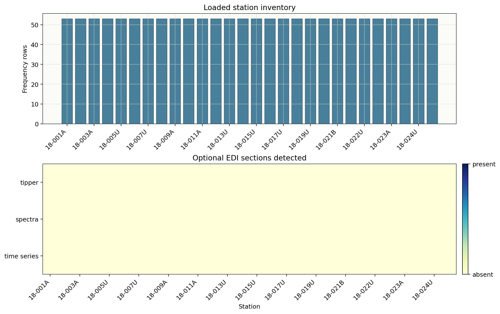
Inventory of the loaded L18PLT line. Station triangles and labels identify the shared columns. The upper markers report 53 rows per station, while the lower map confirms that those rows occupy the same period bands.#
The uniform upper profile rules out isolated loss of complete frequency rows; the uninterrupted lower map additionally rules out hidden station-specific band gaps. The inventory table still shows that optional tipper, spectra, and time-series sections are absent throughout this delivery. Methods requiring those observations are therefore inappropriate unless they are obtained from another source.
2.5.4. Inspect one station#
Before computing line-wide diagnostics, inspect one parsed EDI object:
>>> first = survey[0]
>>> first.station, Path(first.path).name
('23-18-001A', '18-001A.edi')
>>> len(first.Z.freq)
53
>>> survey.get_site("23-18-001A").station
'23-18-001A'
>>> survey.get_site("missing-station") is None
True
The EDI header identity and source filename are related but not identical. Keep both columns when auditing a survey, and do not reconstruct station identity by stripping or adding a filename prefix unless the field metadata documents that convention.
2.5.5. Plot a survey fingerprint#
A compact first diagnostic compares phase-sensitive quantities across station and period. The following public function produces the captured figure:
>>> from pycsamt.emtools import plot_survey_fingerprint
>>> fig = plot_survey_fingerprint(
...     survey.collection,
...     quantities=["skew", "ellipt", "s1"],
...     render="imshow",
...     plot_kws={"interpolation": "bilinear"},
...     station_grid=True,
...     period_range=(1e-4, 1.0),
...     recursive=False,
...     title="L18PLT quick survey fingerprint",
...     figsize=(11.2, 7.6),
... )
>>> len(fig.axes) >= 3
True
The public API defaults to three panels—skew, ellipt, and s1
(\(\phi_{\max}\))—rendered with pcolormesh. This Getting Started view
requests imshow with bilinear interpolation for a visibly continuous
raster presentation. Pass a
single name such as quantities="skew" for one panel, or any ordered subset
such as ["ellipticity", "phi_max"] for two. cmaps accepts either one
colormap or a quantity-to-colormap mapping, while plot_kws and
quantity_kws forward global and per-panel options to the selected
Matplotlib renderer. Contours resolve through the package-wide
pycsamt.api.PYCSAMT_CONTOUR review style by default. Pass
contours=False to hide them, or use contour_kws for a one-call
override. The complete configuration pattern is documented in
Contour overlays.
The dotted vertical guides pass through the same station centre in all three
panels. Set station_grid=False to hide them, or pass
station_grid_kws to control their colour, width, line style, opacity, and
drawing order.
Bilinear interpolation smooths the displayed pixels only; it does not add
measured stations or periods. Use the default pcolormesh view when exact
cell boundaries are important for diagnosis.
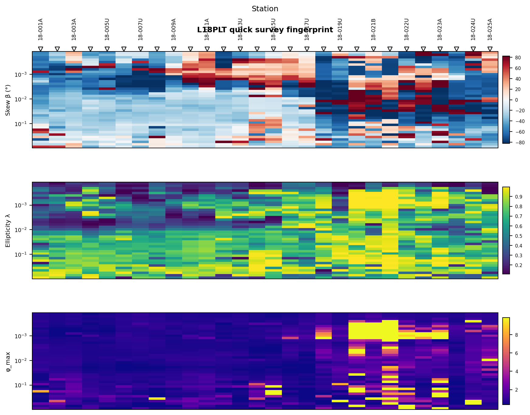
Phase-sensitive fingerprint of the L18PLT survey over periods from \(10^{-4}\) to \(1\) s. Columns are stations and rows are period samples; color represents the quantity shown on each panel.#
The left part of the line is comparatively subdued at short periods, whereas stations in the latter half show strong, coherent changes in skew sign, ellipticity, and the maximum phase-tensor value. Because several quantities change in the same station-period region, the pattern deserves targeted phase-tensor, strike, and source-effect review. It should not be labeled a bad station or a geological boundary from this quick-look figure alone: distortion, three-dimensional structure, noise, and acquisition effects can produce overlapping signatures.
The deterministic generator for the inventory and fingerprint figures is available below. It uses public pyCSAMT interfaces and writes the images into the documentation image tree; user workflows should call those public APIs directly rather than importing this documentation script.
View the figure-generation sourceClick to inspect and copy the complete code
  1#!/usr/bin/env python
  2# Author: LKouadio <etanoyau@gmail.com>
  3# License: LGPL-3.0
  4"""Generate figures and sample outputs for the read-EDI tutorial."""
  5
  6from __future__ import annotations
  7
  8import sys
  9from pathlib import Path
 10
 11import matplotlib
 12
 13matplotlib.use("Agg")
 14
 15import matplotlib.pyplot as plt
 16import numpy as np
 17
 18ROOT = Path(__file__).resolve().parents[2]
 19DATA_DIR = ROOT / "data" / "AMT" / "WILLY_DATA" / "L18PLT"
 20ONE_EDI = DATA_DIR / "18-001A.edi"
 21IMAGE_DIR = (
 22    ROOT / "docs" / "source" / "images" / "tutorials" / "read_edi_survey"
 23)
 24
 25
 26def _import_pycsamt():
 27    """Import the public APIs used by this standalone generator."""
 28    if str(ROOT) not in sys.path:
 29        sys.path.insert(0, str(ROOT))
 30
 31    from pycsamt.api import read_edi, read_edis
 32    from pycsamt.emtools import (
 33        plot_survey_fingerprint,
 34        plot_survey_inventory_overview,
 35    )
 36
 37    return {
 38        "plot_survey_fingerprint": plot_survey_fingerprint,
 39        "plot_survey_inventory_overview": plot_survey_inventory_overview,
 40        "read_edi": read_edi,
 41        "read_edis": read_edis,
 42    }
 43
 44
 45def _style_axis(ax: plt.Axes) -> None:
 46    ax.set_facecolor("#fbfbf7")
 47    ax.grid(True, color="#d8dad1", linewidth=0.7, alpha=0.65)
 48    for spine in ax.spines.values():
 49        spine.set_color("#39434d")
 50        spine.set_linewidth(0.8)
 51
 52
 53def _save(fig: plt.Figure, name: str) -> None:
 54    IMAGE_DIR.mkdir(parents=True, exist_ok=True)
 55    fig.savefig(IMAGE_DIR / name, dpi=180, bbox_inches="tight")
 56    plt.close(fig)
 57
 58
 59def _inventory_plot(functions, survey) -> None:
 60    labels = [name.replace("23-", "") for name in survey.stations]
 61    fig = functions["plot_survey_inventory_overview"](
 62        survey.collection,
 63        station_labels=labels,
 64        recursive=False,
 65        title="L18PLT acquisition inventory and period coverage",
 66        figsize=(11.2, 7.2),
 67    )
 68    _save(fig, "survey_inventory_overview.png")
 69
 70
 71def _path_plot(inventory) -> None:
 72    names = inventory["path"].map(lambda value: Path(value).name)
 73    lengths = names.str.len().to_numpy(dtype=int)
 74    fig, ax = plt.subplots(figsize=(9.0, 3.8))
 75    ax.plot(
 76        np.arange(1, len(names) + 1),
 77        lengths,
 78        color="#7c4d79",
 79        marker="s",
 80        markersize=4,
 81        linewidth=1.2,
 82    )
 83    ax.set_xlabel("Loaded file index")
 84    ax.set_ylabel("Filename length")
 85    ax.set_title("Source filenames are regular across the line")
 86    _style_axis(ax)
 87    _save(fig, "source_filename_check.png")
 88
 89
 90def _fingerprint(functions, survey) -> None:
 91    fig = functions["plot_survey_fingerprint"](
 92        survey.collection,
 93        quantities=["skew", "ellipt", "s1"],
 94        render="imshow",
 95        plot_kws={"interpolation": "bilinear"},
 96        station_grid=True,
 97        period_range=(1e-4, 1.0),
 98        recursive=False,
 99        title="L18PLT quick survey fingerprint",
100        figsize=(11.2, 7.6),
101    )
102    _save(fig, "survey_fingerprint.png")
103
104
105def main() -> int:
106    functions = _import_pycsamt()
107    survey = functions["read_edis"](
108        DATA_DIR,
109        recursive=False,
110        strict=False,
111        on_dup="replace",
112        progress=False,
113    )
114    summary = survey.summary()
115    inventory = summary.to_pandas(copy=True)
116    one = functions["read_edi"](ONE_EDI)
117    single = functions["read_edis"](ONE_EDI, recursive=False, progress=False)
118
119    _inventory_plot(functions, survey)
120    _path_plot(inventory)
121    # Some processing-oriented plotting paths normalize station metadata on
122    # their input collection.  Use a separate load so figure generation cannot
123    # alter the survey used for captured inventory and selection output.
124    plot_survey = functions["read_edis"](
125        DATA_DIR,
126        recursive=False,
127        strict=False,
128        on_dup="replace",
129        progress=False,
130    )
131    _fingerprint(functions, plot_survey)
132
133    print("survey_text:")
134    print(survey)
135    print("survey_properties:")
136    print(f"n_sites={survey.n_sites}")
137    print(f"stations={survey.stations[:5]}")
138    print(f"paths={[Path(p).name for p in survey.paths[:5]]}")
139    print("summary:")
140    print(summary)
141    print("inventory_head:")
142    compact = inventory.copy()
143    compact["path"] = compact["path"].map(lambda value: Path(value).name)
144    print(compact.head(5).to_string(index=False))
145    print(f"columns={inventory.columns.tolist()}")
146    print("single_file:")
147    print(f"read_edi station={one.station}")
148    print(f"read_edis n_sites={single.n_sites}")
149    print(single.summary())
150    print("selection:")
151    first = survey[0]
152    selected = survey.get_site(survey.stations[0])
153    print(f"first={first.station} {Path(first.path).name}")
154    print(f"selected={selected.station} {Path(selected.path).name}")
155    print(f"missing={survey.get_site('S999')}")
156    print("errors:")
157    print(f"{len(survey.errors())} read error(s)")
158    print("focused_table:")
159    focused = survey.summary(
160        fields=["station", "n_freq", "tipper", "path"]
161    ).to_pandas(copy=True)
162    focused["path"] = focused["path"].map(lambda value: Path(value).name)
163    print(focused.head(3).to_string(index=False))
164    print(f"images: {IMAGE_DIR.relative_to(ROOT)}")
165    return 0
166
167
168if __name__ == "__main__":
169    raise SystemExit(main())
2.5.6. Decide whether to continue#
Before processing this or another survey, verify:
the loaded count matches the expected field stations;
every parser error is understood;
station identities map unambiguously to source files;
coordinates and elevation have the expected datum and units;
frequency values—not only their counts—are compatible across stations;
required impedance or tipper components are present;
unusual station-period regions have been reviewed with more specific diagnostics.
Warning
A complete inventory and an attractive diagnostic plot do not establish inversion readiness. Static shift, dead bands, source effects, coordinate errors, uncertainty estimates, and dimensionality assumptions require separate checks.
Continue to Read an EDI Survey for deeper EDI inspection or Inspect and QC a Survey for quality-control diagnostics. The reusable loading and normalization rules are summarized in Loading electromagnetic data; processing methods are organized under EM Tools Guide.