
18.4. Compare Survey Lines for QC#
This tutorial shows how to compare two EDI survey lines before applying the same processing workflow to both. It is useful when a project has several parallel lines, adjacent profiles, or repeat surveys and you need to decide whether one first-pass QC configuration is defensible.
The example uses the bundled L18PLT and L22PLT lines:
data/AMT/WILLY_DATA/L18PLTdata/AMT/WILLY_DATA/L22PLT
The goal is not to prove that the two lines are geologically identical. The goal is more practical: check whether the input structure, frequency coverage, and first-pass quality metrics are similar enough to start with the same QC pipeline, while still estimating line-specific corrections later.
18.4.1. What You Will Learn#
After this tutorial you should be able to:
load two EDI line folders;
build comparable station inventories;
compare station count, frequency rows, and optional EDI sections;
compare frequency-band overlap;
compute QC and confidence summaries by line;
decide whether one first-pass config can be reused;
adapt the same pattern to your own EDI data.
18.4.2. Input Assumptions#
The examples below assume that the two line folders are available in the repository sample data:
data/
  AMT/
    WILLY_DATA/
      L18PLT/
        18-001A.edi
        ...
      L22PLT/
        22-10U.edi
        ...
For your own project, replace these two paths with your line directories. Keep the line labels short, because they will be used in tables and plot legends.
18.4.3. Load Both Lines#
Start with pycsamt.api.read_edis() for each line:
>>> from pathlib import Path
>>> from pycsamt.api import read_edis
>>> lines = {
...     "L18PLT": Path("data/AMT/WILLY_DATA/L18PLT"),
...     "L22PLT": Path("data/AMT/WILLY_DATA/L22PLT"),
... }
>>> surveys = {
...     name: read_edis(
...         path,
...         recursive=False,
...         strict=False,
...         on_dup="replace",
...         progress=False,
...     )
...     for name, path in lines.items()
... }
>>> for name, survey in surveys.items():
...     print(name, survey.summary())
L18PLT APIFrame: edi_survey_summary
kind: edi.summary
shape: 28 rows x 6 columns
columns: station, path, n_freq, tipper, spectra, ts
numeric: 1 columns
missing: 0.0%
source: data\AMT\WILLY_DATA\L18PLT
L22PLT APIFrame: edi_survey_summary
kind: edi.summary
shape: 25 rows x 6 columns
columns: station, path, n_freq, tipper, spectra, ts
numeric: 1 columns
missing: 0.0%
source: data\AMT\WILLY_DATA\L22PLT
The survey object keeps the public loading summary, while
survey.collection is the lower-level object used by the QC functions.
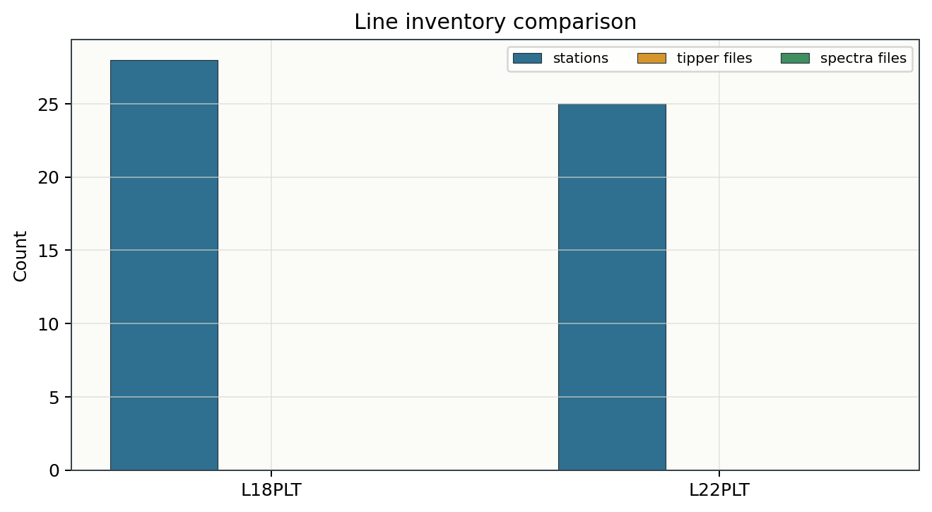
Already visible here: L18PLT has 28 stations and L22PLT has 25 –
close enough that a shared review process is plausible, but different
enough that the two lines are not simply the same survey split in half.
18.4.4. Build Comparable Inventory Tables#
The first check is structural: number of stations, number of frequency rows, and whether optional EDI sections such as tipper or spectra are present.
>>> import pandas as pd
>>> inventories = []
>>> for name, survey in surveys.items():
...     table = survey.summary().to_pandas(copy=True)
...     table["line"] = name
...     inventories.append(table)
>>> inventory = pd.concat(inventories, ignore_index=True)
>>> cols = ["line", "station", "n_freq", "tipper", "spectra"]
>>> print(inventory[cols].head(6).to_string(index=False))
  line    station  n_freq  tipper  spectra
L18PLT 23-18-001A      53   False    False
L18PLT 23-18-002U      53   False    False
L18PLT 23-18-003A      53   False    False
L18PLT 23-18-004A      53   False    False
L18PLT 23-18-005U      53   False    False
L18PLT 23-18-006A      53   False    False
>>> inventory["tipper"].any(), inventory["spectra"].any()
(False, False)
For the bundled data, both lines have a regular EDI structure and the same
number of frequency rows per station. Neither line carries tipper or
spectra sections at all – tipper/spectra are False for every
row on both lines, not just the six shown here. That matters for the figure
below: its “tipper files” and “spectra files” bars are genuinely zero for
this bundled AMT data, not a rendering artifact, so on this dataset the
comparison reduces to station counts. On a survey where tipper or spectra
data exist, the same two bars would carry real information about which line
has fuller instrument coverage.
18.4.5. Compare Frequency Coverage#
Before reusing a frequency-band parameter, compare the effective frequency
range. The QC table contains period limits, so frequency limits can be derived
from pmax and pmin:
>>> from pycsamt.emtools.qc import build_qc_table
>>> qc_tables = []
>>> for name, survey in surveys.items():
...     qc = build_qc_table(
...         survey.collection,
...         include_skew=True,
...         recursive=False,
...         api=True,
...     ).to_pandas(copy=True)
...     qc["line"] = name
...     qc_tables.append(qc)
>>> qc = pd.concat(qc_tables, ignore_index=True)
>>> frequency_summary = qc.groupby("line").agg(
...     min_freq_hz=("pmax", lambda value: 1.0 / value.max()),
...     max_freq_hz=("pmin", lambda value: 1.0 / value.min()),
...     median_frac_ok=("frac_ok", "median"),
... )
>>> print(frequency_summary.to_string(float_format=lambda v: f"{v:.3g}"))
        min_freq_hz  max_freq_hz  median_frac_ok
line
L18PLT         1.01     1.04e+04               1
L22PLT         1.01     1.04e+04               1
The two bundled lines share essentially the same first-pass band – to six
significant figures, the same min_freq_hz/max_freq_hz bounds, and
every station on both lines has frac_ok=1.0. This supports using the
same initial select_band setting for both lines, for example
band_hz: [1.0, 10000.0]. A shared band is a necessary check, not a
sufficient one – two lines can share an identical frequency range while
still differing in how much of that range is actually trustworthy, which is
exactly what the confidence comparison below tests next.
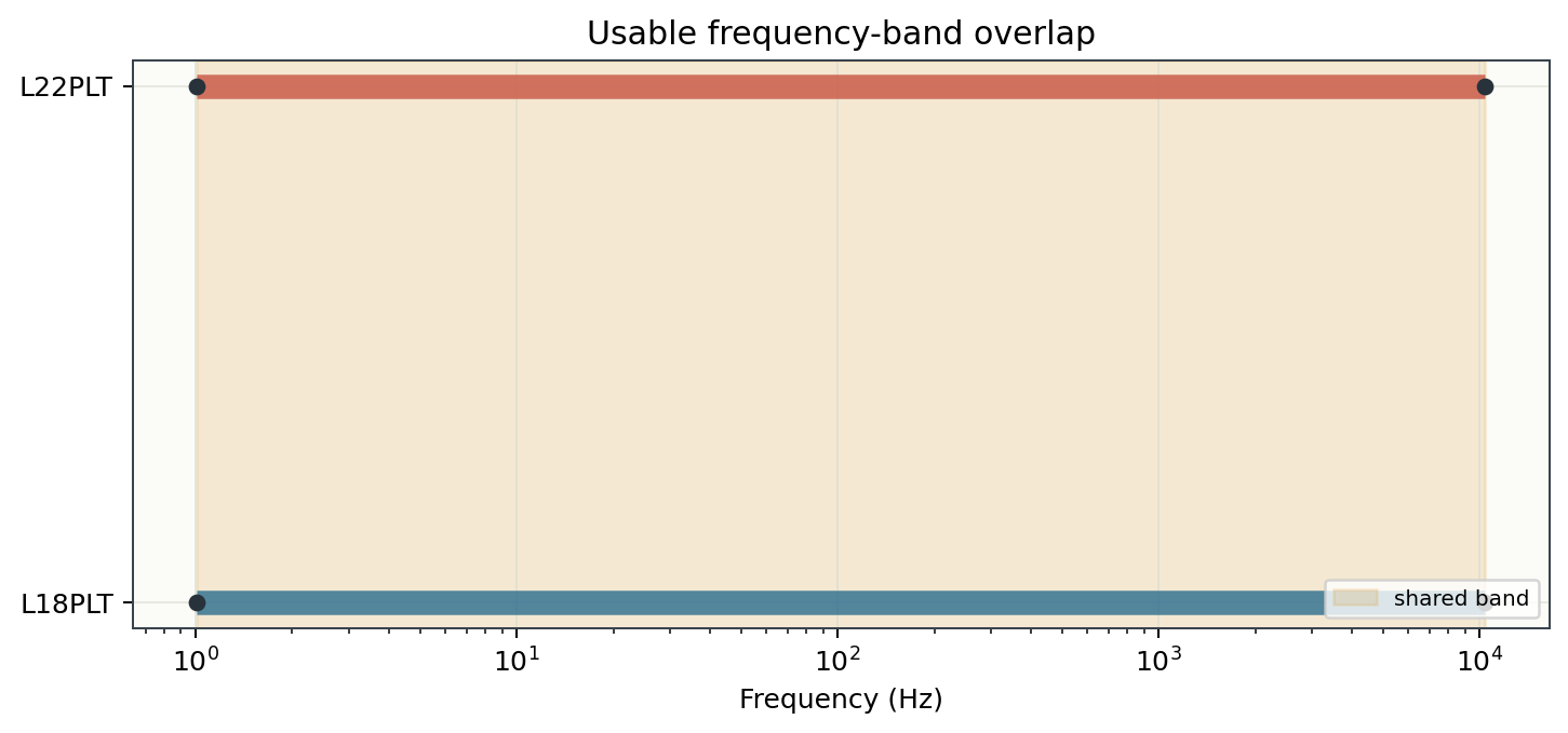
The two horizontal bars span the same log-frequency range and the shaded
“shared band” region covers essentially the full length of both – a visual
match for the near-identical min_freq_hz/max_freq_hz values above.
When two lines instead show bars that only partially overlap, the shaded
region marks the safe common band; anything outside it needs a per-line
frequency choice rather than one shared setting.
18.4.6. Compare QC and Confidence Metrics#
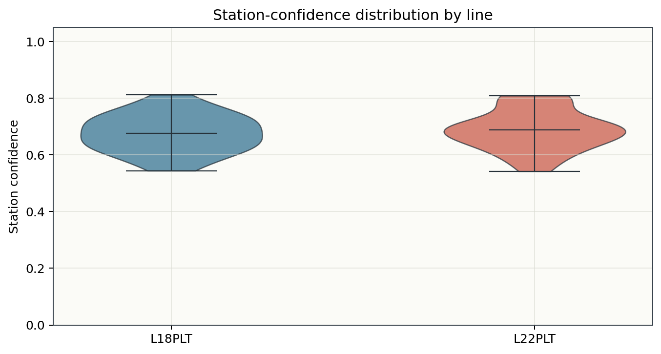
Frequency coverage is necessary, but not sufficient. Compare station-level quality metrics before deciding that a shared workflow is reasonable:
>>> from pycsamt.emtools.qc import station_confidence_table
>>> confidence_tables = []
>>> for name, survey in surveys.items():
...     confidence = station_confidence_table(
...         survey.collection,
...         method="composite",
...         relerr_threshold=0.20,
...         offdiag_tolerance_log10=0.35,
...         diagonal_leakage_max=0.35,
...         phase_jump_tolerance_deg=90.0,
...         spatial_tolerance_log10=0.60,
...         spacing_m=200.0,
...         recursive=False,
...         api=True,
...     ).to_pandas(copy=True)
...     confidence["line"] = name
...     confidence_tables.append(confidence)
>>> confidence = pd.concat(confidence_tables, ignore_index=True)
>>> ci_summary = confidence.groupby("line").agg(
...     stations=("station", "count"),
...     confidence_min=("confidence", "min"),
...     confidence_median=("confidence", "median"),
...     confidence_max=("confidence", "max"),
... )
>>> print(ci_summary.to_string(float_format=lambda v: f"{v:.3f}"))
        stations  confidence_min  confidence_median  confidence_max
line
L18PLT        28           0.544              0.672           0.812
L22PLT        25           0.542              0.699           0.809
The medians are close (0.672 vs 0.699) but not identical, and the
minimums are almost the same (0.544 vs 0.542) while the maximums
differ by only 0.003. That is the useful answer: the same first-pass QC
config is reasonable for both lines – neither line is systematically
worse, and both span a similar confidence range – but any station
rejection, static-shift correction, or inversion weighting should still be
reviewed per line rather than assumed identical, since a matching range
does not mean the same stations within each line are the weak ones.
18.4.7. Make the Processing Decision#
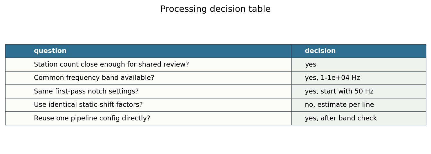
Summarise the comparison as a decision table. This is the part worth keeping in a project note or reviewer response, because it explains why you reused a workflow or why you did not.
>>> line_summary = pd.DataFrame(
...     [
...         {
...             "line": name,
...             "stations": len(surveys[name].summary().to_pandas()),
...             "median_n_freq": inventory.loc[
...                 inventory["line"] == name, "n_freq"
...             ].median(),
...             "median_frac_ok": qc.loc[
...                 qc["line"] == name, "frac_ok"
...             ].median(),
...             "median_confidence": confidence.loc[
...                 confidence["line"] == name, "confidence"
...             ].median(),
...         }
...         for name in surveys
...     ]
... )
>>> print(line_summary.round(3).to_string(index=False))
  line  stations  median_n_freq  median_frac_ok  median_confidence
L18PLT        28           53.0             1.0              0.672
L22PLT        25           53.0             1.0              0.699
For these two lines, a practical decision is:
reuse the same first-pass QC and frequency-band config;
keep the line labels separate in all outputs;
estimate static-shift factors separately for each line;
review stations with low confidence before inversion preparation;
do not merge the lines unless the modelling objective requires it.
18.4.8. Recommended Next Step#
Once the comparison supports a shared first-pass workflow, run the config pipeline separately for each line:
1pycsamt pipe run \
2    --config config/l18_first_qc.yaml \
3    --survey data/AMT/WILLY_DATA/L18PLT \
4    --out results/L18PLT_first_qc
5
6pycsamt pipe run \
7    --config config/l18_first_qc.yaml \
8    --survey data/AMT/WILLY_DATA/L22PLT \
9    --out results/L22PLT_first_qc
Using the same config does not mean mixing the outputs. Keep one output folder per line so that plots, processed EDIs, reports, and later inversion files stay traceable.
18.4.9. Adapting This Tutorial#
For your own data, replace only the lines dictionary:
1lines = {
2    "Line_A": Path("path/to/line_a_edis"),
3    "Line_B": Path("path/to/line_b_edis"),
4}
Then rerun the same inventory, QC, confidence, and decision-table steps. If the
frequency bands differ, use separate select_band parameters. If confidence
distributions differ strongly, inspect the weaker line before applying
corrections or preparing inversion input.
18.4.10. See Also#
- Read an EDI Survey
Load EDI surveys and inspect the public survey object.
- Inspect and QC a Survey
Build detailed QC tables and diagnostic plots for one line.
- Run a Pipeline From Config
Store the resulting first-pass workflow in a reusable config file.
- Correct Static Shift
Estimate static-shift factors after the QC decision is understood.