6.3.1. AI inversion concepts#

AI inversion estimates an earth model from electromagnetic observations with a learned or differentiable computational model. In pyCSAMT, this includes three related approaches:

supervised AI inversion, which learns from synthetic response–model pairs;
physics-informed inversion, which optimizes model parameters through a differentiable forward-physics loss without labelled earth models;
hybrid inversion, which uses an AI estimate as a starting point or model prior for subsequent physics-based refinement.

These approaches can make repeated inversion fast, provide useful screening models, and support uncertainty experiments. They do not remove the non-uniqueness of electromagnetic inversion. Their results remain conditional on data quality, parameterization, physics, training coverage, regularization, and validation evidence.

Core principle

A neural network does not learn “the subsurface.” It learns a relationship defined by its inputs, targets, forward simulator, parameter ranges, loss, architecture, and training examples. A field prediction is defensible only to the extent that this learned relationship represents the survey.

6.3.1.1. Where AI inversion fits#

The principal EM workflow is:

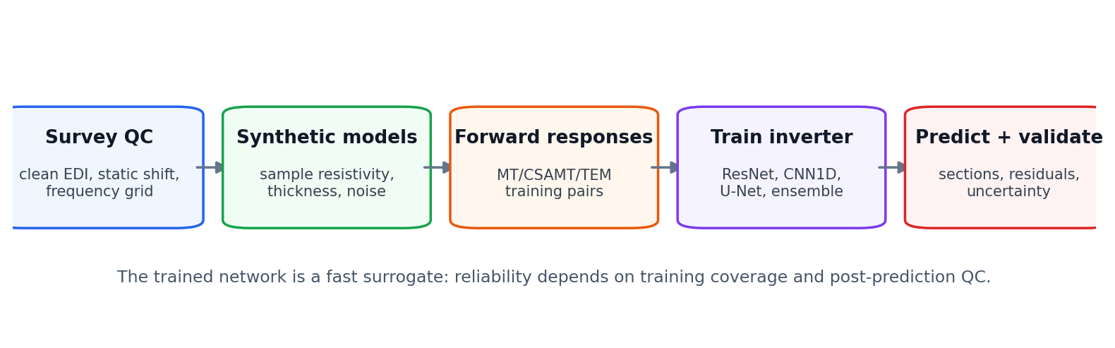
Relationship among field data, forward modeling, AI inversion, validation, and interpretation — Forward modeling supplies controlled response–model relationships. AI inversion predicts candidate models. Response reconstruction, uncertainty, classical baselines, and independent evidence determine whether those candidates are suitable for interpretation.#

The stages have distinct roles:

Forward modeling: Predicts observations \(\mathbf d\) from an earth model \(\mathbf m\) through the forward operator \(\mathbf d=F(\mathbf m)\).
Classical inversion: Searches for a model by repeatedly evaluating physics and minimizing an objective such as data misfit plus regularization.
Supervised AI inversion: Learns an approximation \(G_\theta\) to the inverse relationship from examples and predicts \(\hat{\mathbf m}=G_\theta(\mathbf d)\). Training pays the repeated optimization cost in advance, so applying the fitted map to another compatible observation is an amortized inversion.
Physics-informed inversion: Uses differentiable physics during optimization, often minimizing \(\|F(\mathbf m_\theta)-\mathbf d_{\mathrm{obs}}\|\) plus constraints.
Interpretation: Connects the reviewed resistivity model to geology or hydrogeology. It is not part of network prediction and requires additional evidence.

6.3.1.2. Why EM inversion remains difficult#

Electromagnetic inversion is nonlinear and ill posed. Different resistivity models can produce responses that are indistinguishable within measurement error. Sensitivity changes with period, depth, component, geometry, and conductivity structure. Finite bandwidth limits depth resolution, while noise, distortion, source effects, and dimensionality violations introduce additional ambiguity.

Classical inversion manages this with regularization, error models, starting models, constraints, and model appraisal. Supervised AI manages it implicitly through the training distribution, target representation, loss, architecture, and data augmentation. Those choices are forms of prior information even when they are not called regularization.

Consequently:

a single response need not have a single correct target model;
a low supervised test error can coexist with field failure;
a smooth prediction may reflect training targets rather than geology;
network confidence can be high outside the supported domain;
fast inference changes computational cost, not physical information content.

6.3.1.3. Three AI inversion families#

Supervised surrogate inversion#

The supervised workflow samples earth models from a chosen model prior, calculates synthetic responses, and fits a network to recover the sampled parameters. If \(p(\mathbf m)\) is the model-sampling law and \(p(\boldsymbol\epsilon\mid\mathbf m)\) describes the noise model, each training pair is generated as

(1)#\[\mathbf d_i = F(\mathbf m_i) + \boldsymbol\epsilon_i, \qquad \mathbf m_i \sim p(\mathbf m).\]

The learned map \(G_\theta\) is therefore tied to the sampled resistivities, thicknesses, geometry, frequency grid, components, and noise that produced those pairs. pyCSAMT provides:

pycsamt.ai.inversion.EMInverter1D;
pycsamt.ai.inversion.EMInverter2D;
pycsamt.ai.inversion.GCNInverter3D;
pycsamt.ai.inversion.JointInverter;
pycsamt.ai.inversion.EnsembleInverter.

Advantages include rapid inference after training, consistent execution across many stations, and direct access to synthetic ground truth during development. The principal risk is the simulation-to-field domain gap.

Physics-informed inversion#

pyCSAMT exposes:

These approaches optimize through a physics loss and do not require labelled training models in the same way as supervised inversion. A network or differentiable parameterization \(\mathbf m_\theta\) is adjusted until its forward response resembles the observation. They still depend on the selected forward operator, model parameterization, regularization weights, boundary assumptions, optimizer, and stopping rule. “Physics-informed” does not mean exact physics or unique recovery.

Hybrid inversion#

pyCSAMT provides:

Hybrid inversion combines learned speed with physics-based correction. For example, an AI result can initialize an iterative refinement. This can reduce runtime or starting-model sensitivity, but refinement cannot rescue an incompatible parameterization or missing physics automatically.

6.3.1.4. Choosing 1-D, 2-D, or 3-D#

Dimension describes the model and information-sharing assumption, not merely the shape of an output array.

Level	Representation	Appropriate context	Principal risk
1-D	One layered model per sounding.	Locally layered earth, sparse surveys, rapid station screening, or a baseline before higher-dimensional analysis.	Lateral structure is mapped into misleading layer parameters.
2-D	A depth–station section predicted from an ordered profile panel.	A line survey whose strike and dimensionality evidence support a 2-D approximation.	A tiled 1-D training set, a genuine 2-D Maxwell training set, and a classical 2-D field inversion are treated as interchangeable.
Graph 3-D	Layered station parameters share information through a spatial graph.	Multi-line or areal surveys with reviewed coordinates and meaningful neighborhood relationships.	Graph context, genuine 3-D training physics, and a classical 3-D field inversion are presented as though they were the same operation.

GCNInverter3D is graph-context inversion. It predicts layered parameters at spatial stations and shares information through adjacency. With Inv3DAgent(physics="mt1d"), its responses remain tiled layered-earth simulations. With physics="mt3d", correlated 3-D volumes are solved by MT3DAdapter before training, so lateral and vertical conductivity contrasts enter the same forward solve. The inverse architecture remains a GCN in both cases; training with 3-D physics does not turn it into an iterative ModEM field inversion or validate an arbitrary field prediction.

Select dimension using strike, dimensionality, tipper behavior, survey geometry, target geometry, station spacing, and classical response evidence—not because a higher number sounds more advanced.

6.3.1.5. Depth support is not the model depth#

An AMT frequency band does not define a sharp maximum depth. For a uniform earth, the skin depth gives the electromagnetic attenuation scale

(2)#\[\delta(f,\rho) = \sqrt{\frac{2\rho}{\mu_0\,2\pi f}} \simeq 503\sqrt{\frac{\rho}{f}}\ \mathrm{m},\]

where \(f\) is frequency in hertz, \(\rho\) is resistivity in ohm metres, and \(\mu_0\) is the free-space magnetic permeability. Equation (2) describes attenuation in a homogeneous conductor. It is not a depth of investigation, a vertical-resolution estimate, or permission to train an inverter to that depth. In a layered earth, conductive cover can screen deeper structure, resistive material can inflate the scale, and sensitivity decays gradually rather than stopping at \(\delta\).

The bundled WILLY L18 profile makes the difference concrete. The following diagnostic reads all 28 stations and deliberately computes only a skin-depth scale from the observed XY apparent resistivity. It does not invert the data.

>>> import numpy as np
>>> from pycsamt.emtools._core import ensure_sites
>>> from pycsamt.ai.inversion import sites_to_obs_1d

>>> sites = ensure_sites(
...     "data/AMT/WILLY_data/L18PLT", recursive=True, verbose=0
... )
>>> obs = sites_to_obs_1d(sites, comp="xy")
>>> frequency_hz = np.asarray(obs[0].freq)
>>> rho_a = np.vstack([item.rho_obs for item in obs])
>>> rho_median = np.nanmedian(rho_a, axis=0)
>>> delta_m = 503.0 * np.sqrt(rho_median / frequency_hz)
>>> print(f"stations={len(obs)}, frequencies={frequency_hz.size}")
stations=28, frequencies=53
>>> print(f"frequency range={frequency_hz.min():.3f}--{frequency_hz.max():.0f} Hz")
frequency range=1.008--10400 Hz
>>> i = int(np.nanargmin(frequency_hz))
>>> print(f"lowest-frequency skin-depth scale={delta_m[i] / 1000:.1f} km")
lowest-frequency skin-depth scale=30.7 km

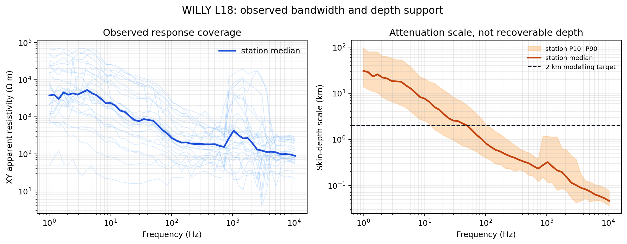
WILLY L18 apparent-resistivity coverage and skin-depth diagnostic — The left panel shows the actual XY apparent-resistivity curves and their station median. The right panel translates them through equation (2); the broad band is variation among stations, not an uncertainty interval. The 2 km line is a conservative modelling target, not a boundary inferred from the crossing.#

The 30.7 km value is therefore a warning against equating penetration with resolution. For an expected target shallower than 2 km, set the synthetic model bottom somewhat below the target so boundary conditions do not control it, but report interpretation only where response sensitivity, perturbation or Jacobian tests, recovery experiments, error-aware forward reconstruction, and independent evidence agree. Training labels below that supported interval teach the network a prior; the field data do not turn those labels into observations.

6.3.1.6. Model parameterization#

The network can only recover parameters represented in its output.

Layered 1-D target#

A common target vector contains n_layers resistivities and n_layers - 1 thicknesses:

y = [log10(rho_1), ..., log10(rho_L),
     log10(h_1), ..., log10(h_(L-1))]

Resistivity is commonly expressed in ohm metres and thickness in metres before the base-10 logarithm is taken. With \(L\) layers, the target dimension is \(2L-1\) because the bottom half-space has no thickness. Inverting the transformed output returns \(\rho_\ell=10^{y_\ell}\) and \(h_\ell=10^{y_{L+\ell}}\). Increasing layer count increases flexibility but also ambiguity and training difficulty.

Fixed-grid 2-D target#

A profile inverter may predict log10(rho) on a fixed (n_depth, n_stations) grid. Depth discretization is then part of the model prior. A visually sharp boundary cannot be more resolved than the information in the responses and training examples. pyCSAMT’s 2-D U-Net can be trained either on a pseudo-2-D training model made by tiling independent 1-D responses or on 2-D Maxwell training model realizations containing lateral TE coupling. Both produce the same target-array shape; the shape alone does not disclose which physics generated it. Preserve physics, solver identity, mesh controls, components, and spatial correlation parameters with the checkpoint.

Graph target#

Graph inversion commonly predicts the layered target at every station. A later volume or depth slice interpolates these predictions spatially. Separate network output, graph smoothing, and post-prediction gridding in reports.

For genuine MT3D training, the resistivity label at station \(s\) is the vertical column sampled from the same realization \(r\) that generated its response,

(3)#\[y_{r,s,k} =\log_{10}\rho_r \left(x_{j(s)},y_{q(s)},z_{p(k)}\right),\]

where \(j(s)\) and \(q(s)\) select the nearest geology-grid column and \(p(k)\) maps the requested output layer to a geology-grid depth. Equation (3) is a nearest-cell sampling contract; it does not create finer geological information when the output grid contains more layers than the training geology grid.

Three grids in a 3-D AI workflow#

A robust 3-D workflow keeps three discretizations distinct:

Geology grid: Stores the sampled true resistivity volume and defines the spatial support of interfaces, correlations, or bodies. In the built-in dataset generator, this is a comparatively coarse GeologyGrid.
Solver mesh: Discretizes Maxwell’s equations. It may add fine core cells and geometrically growing padding around the geology domain. The current research MT3D path supports a non-uniform tensor mesh, so physical extent and local resolution need not be forced into one uniform cell size.
Inverse-output grid: Contains the station-layer values predicted by the GCN. It is fixed by station coordinates, n_layers, and depth_max; spatial interpolation into a display volume occurs only afterward.

Let \(P_{g\rightarrow s}\) map geology-cell conductivity to the solver mesh, \(F_s\) denote the discrete Maxwell solve, and \(P_{g\rightarrow o}\) sample geology columns onto the inverse-output layers. One supervised realization is therefore

(4)#\[\mathbf d_r =F_s\!\left(P_{g\rightarrow s}\boldsymbol\sigma_r\right), \qquad \mathbf y_r =P_{g\rightarrow o}\log_{10}\boldsymbol\rho_r.\]

The two mappings in equation (4) serve different purposes and must be preserved in provenance. Treating a padded solver mesh as though it were the geological truth changes labels; treating an interpolated output volume as though it were directly solved invents spatial resolution.

Topography adds another boundary decision. A terrain-draped section may use measured elevation only to transform depth below ground into an absolute vertical coordinate. Terrain affects physics only when earth, air, receivers, and conductivity are mapped consistently onto a solver that supports that topographic contract. The current Inv3DAgent records affects_forward_physics=False for its draped output.

Parameterization decisions include:

linear versus logarithmic variables;
bounds and probability distributions;
number and thickness of layers or depth cells;
fixed versus predicted interfaces;
anisotropy or isotropy;
components and modes represented;
topography, source, and distortion parameters;
whether properties vary independently or through geological rules.

6.3.1.7. Data representation#

The input representation determines what the network can use. In pyCSAMT this is the feature vector or matrix handed to the learned model.

Possible features include:

log10 apparent resistivity;
phase;
real and imaginary impedance components;
TE/TM or tensor-component combinations;
TDEM decay values;
frequency or period coordinates;
masks, errors, and quality indicators;
station coordinates or adjacency.

The same observed data can yield different learned problems depending on feature choice. Apparent resistivity and phase are derived from impedance; treating all of them as independent channels can duplicate information.

pyCSAMT provides public bridge utilities rather than requiring invented field feature helpers:

These utilities help enforce the contract between pycsamt.site.Sites and AI arrays. Their outputs still need review for station order, component, frequency coverage, masking, and finite values.

For the 1-D bridge, the common grid contains \(n_f\) logarithmically spaced frequencies between either the observed extrema or explicit freq_min and freq_max. At each station, interpolation is linear in log-frequency; log apparent resistivity and phase are interpolated separately,

(5)#\[\begin{split}x_{s,q} = \begin{cases} \mathcal I_{\log f}\!\left[\log_{10}\rho_{a,s}\right](f_q), &0\le q<n_f,\\ \mathcal I_{\log f}\!\left[\phi_s\right](f_{q-n_f}), &n_f\le q<2n_f, \end{cases}\end{split}\]

where \(s\) identifies the station and \(\mathcal I_{\log f}\) is piecewise-linear interpolation on \(\log_{10}f\). Values outside a station’s own measured interval are NaN rather than extrapolated. Thus a grid lying inside the survey-wide range can still contain missing values for stations with narrower coverage. sites_to_features_1d preserves those NaN values, while obs_to_features_1d currently replaces missing log resistivity by 2 and missing phase by 45 degrees. These two helpers are not semantically interchangeable merely because their returned shapes match.

6.3.1.8. The feature contract#

The feature contract is the reproducibility boundary between a checkpoint and the data sent into it. Training and inference must use the same:

feature names and order;
units and transformations;
frequency or period grid;
component convention;
interpolation method;
missing-value and mask behavior;
normalization statistics;
station ordering and padding policy;
coordinate units and adjacency rules.

A checkpoint without its feature contract is incomplete. A matrix with the right shape but wrong channel order can produce plausible yet meaningless predictions.

6.3.1.9. Training distribution as prior#

The training distribution defines which earth structures the network expects. It therefore acts as an implicit prior.

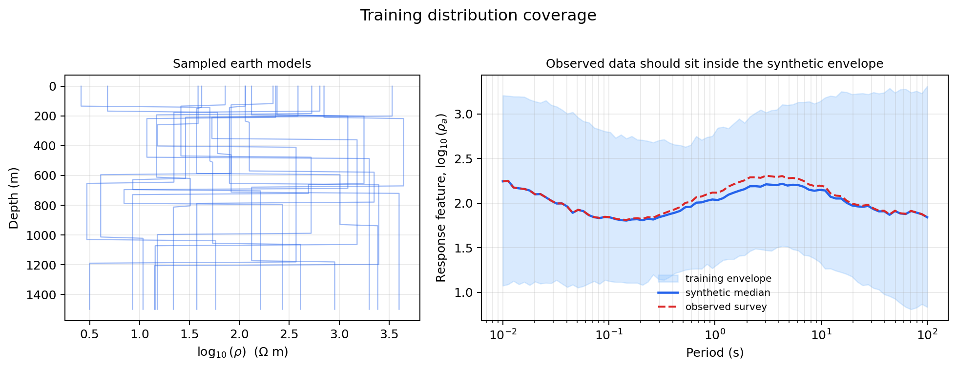
Comparison of synthetic training coverage and field observations — Field responses outside the synthetic envelope require extrapolation. Network behavior there is not validated by ordinary held-out synthetic performance.#

Design choices include:

Geology: Resistivity ranges, layer counts, thicknesses, correlations, interfaces, faults, lateral structures, anisotropy, and rare targets. The built-in 3-D Maxwell dataset currently samples correlated Gaussian volumes; explicit layers, lenses, contacts, and multiple-body families require an externally assembled geology corpus. More realizations of one family do not broaden that family.
Survey: Frequency range, sampling density, station count, spacing, line layout, components, source geometry, and coordinate uncertainty.
Noise and nuisance effects: Heteroscedastic errors, missing bands, outliers, static shift, source effects, cultural noise, distortion, and processing variability.
Physics: Forward solver, dimensionality, boundary conditions, mesh accuracy, and approximations. Record the exact backend: the research-scale in-process MT3DAdapter and the compiled production ModEm3DAdapter solve the same governing physics under different numerical and capability contracts.
Class balance: Frequency of common backgrounds versus rare conductive or resistive targets.

Sampling parameters independently from broad uniform ranges is convenient but may create geologically impossible examples. Conversely, an overly narrow geological generator can produce excellent test metrics and poor field coverage.

6.3.1.10. Simulation-to-field domain gap#

The domain gap is the difference between synthetic training examples and field observations. Sources include:

incomplete forward physics;
wrong dimensionality;
underestimated noise and missing data;
static shift and galvanic distortion;
source and near-field effects;
topography and anisotropy;
coordinate and instrument errors;
processing differences;
geology outside sampled priors.

Good synthetic validation does not measure this gap. Diagnose it by comparing feature distributions, response envelopes, residual patterns, classical inversions, and independent field evidence. Fine-tuning on field labels can help only when trustworthy labels exist and leakage is controlled.

6.3.1.11. Supervised learning objective#

A supervised inverter minimizes a model-space metric over examples:

(6)#\[\mathcal L_{\mathrm{model}}(\theta) = \frac{1}{N}\sum_i \ell\!\left(G_\theta(\mathbf d_i),\mathbf m_i\right).\]

Equation (6) rewards resemblance to the selected synthetic target, but does not guarantee that the predicted model reconstructs the field response. A stronger workflow also evaluates a response-space metric:

(7)#\[\mathcal L_{\mathrm{data}} = \left\|\mathbf W_d \left(F(\hat{\mathbf m})-\mathbf d_{\mathrm{obs}}\right)\right\|_2^2.\]

In equation (7), \(\mathbf W_d\) is usually built from data standard deviations or quality weights, so high-uncertainty observations carry less influence than well-constrained ones. The forward operator, error weights, components, and residual space must be stated. An unweighted RMS misfit of log apparent resistivity is not equivalent to a full complex-impedance likelihood.

6.3.1.12. Physics-informed objective#

A PINN-style objective can combine data fit and regularization:

(8)#\[\mathcal L(\theta) = \mathcal L_{\mathrm{data}}(\theta) + \lambda_v\mathcal R_v(\mathbf m_\theta) + \lambda_l\mathcal R_l(\mathbf m_\theta) + \lambda_g\mathcal R_g(\mathbf m_\theta),\]

In equation (8), vertical, lateral, or graph regularizers apply according to dimension. The weights determine the balance between fit and structure. They must be treated as inversion parameters and tested, not hidden as neural-network details.

6.3.1.13. Architectures encode assumptions#

Fully connected network: Treats the feature vector globally. It is simple but does not explicitly encode local frequency structure.
1-D convolution: Learns local patterns along an ordered feature or frequency axis. Channel arrangement and padding affect meaning.
Residual network: Uses skip connections to train deeper transformations and often provides a strong station-level baseline.
U-Net: Combines local convolution and multiscale skip connections for profile panels. Its receptive field encourages lateral continuity. The network is not itself a classical 2-D EM solver, although its synthetic training responses may now be generated with the 2-D Maxwell adapter rather than tiled 1-D columns.
Graph convolutional network: Propagates information along an adjacency graph. Radius, coordinate system, normalization, and graph connectivity become inversion assumptions. The graph architecture determines information sharing; physics="mt1d" or physics="mt3d" determines how supervised responses were generated.

Architecture comparison is valid only when datasets, splits, preprocessing, target scale, training budget, and selection procedure are controlled.

6.3.1.14. Training, validation, and test separation#

Use distinct roles:

Training set: Updates network parameters.
Validation set: Selects epochs, hyperparameters, and checkpoints.
Calibration set: Fits conformal or posterior calibration without changing the base network.
Synthetic test set: Estimates final performance on unseen synthetic cases.
Field validation set: Tests transfer using observations or independent constraints not used in training, tuning, or calibration.

Random row splitting can leak nearly identical models or profiles across sets. Prefer group splitting by geological scenario, profile family, random generator seed, or survey realization. For spatial field data, nearby stations are not independent test samples when the model shares spatial information.

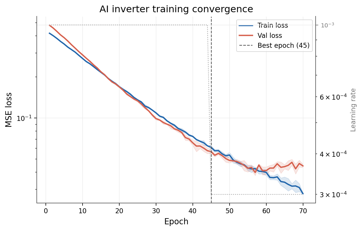
Training and validation loss showing checkpoint selection — Training loss measures optimization on seen examples. Validation divergence can indicate overfitting, but parallel curves do not prove field transfer.#

6.3.1.15. Evaluation hierarchy#

Evaluate at several levels:

Model-space metrics: Error in log resistivity, thickness, boundary depth, or complete sections on synthetic cases with known truth.
Response-space metrics: Difference between observed responses and responses recomputed from the prediction. The reconstruction must match the claimed dimensionality: an MT1D response computed independently at each station is a useful screen but is not a coupled 3-D response validation.
Structural metrics: Boundary location, anomaly continuity, target detection, volume overlap, or graph consistency where scientifically relevant.
Calibration metrics: Interval coverage, reliability, and sharpness on held-out calibration/test data.
Out-of-distribution diagnostics: Distance or coverage relative to synthetic inputs and latent representations.
Field baselines: Bostick-style transforms, classical 1-D/2-D/3-D inversion, boreholes, mapped geology, and other geophysics.
Decision metrics: Whether target ranking, boundary depth, or classification remains correct under accepted uncertainty and scenarios.

No single metric is sufficient. A low model-space error can hide response mismatch, and a low response residual can correspond to the wrong model because the inverse problem is non-unique.

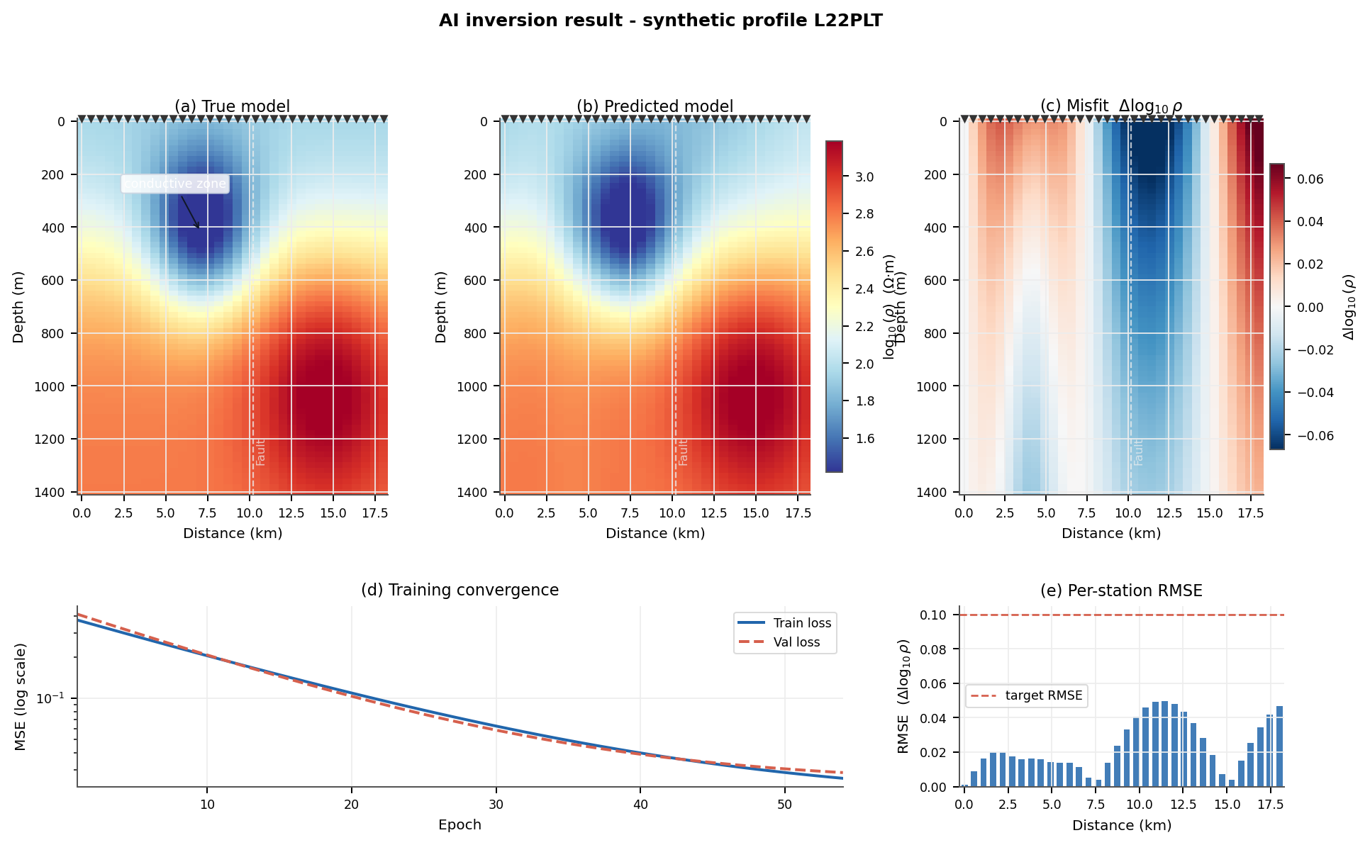
Predicted AI resistivity section displayed with residual and review diagnostics — Review predictions together with coverage, response reconstruction, residuals, uncertainty, and classical or geological evidence.#

6.3.1.16. Uncertainty concepts#

Useful distinctions are:

Aleatoric uncertainty: Variation associated with observation noise or irreducible ambiguity.
Epistemic uncertainty: Uncertainty in learned parameters due to finite or incomplete training data.
Distributional uncertainty: Risk that the field input comes from a different distribution than training.
Inverse non-uniqueness: Multiple earth models fit the observations. A deterministic network can collapse these possibilities into one conditional estimate.
Structural uncertainty: Wrong dimension, parameterization, forward physics, architecture, or geological assumptions.

pyCSAMT exposes pycsamt.ai.inversion.EnsembleInverter, pycsamt.ai.inversion.ConformalPredictor, pycsamt.ai.inversion.PosteriorCalibrator, and MC-dropout prediction for the graph inverter. Each covers only part of this taxonomy.

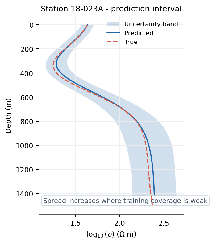
Predictive interval widening with depth — Predictive spread should be interpreted conditionally on the ensemble, calibration set, or dropout model that produced it.#

Conformal coverage applies under exchangeability assumptions between calibration and future examples. Synthetic calibration does not guarantee the same coverage on shifted field data. Narrow intervals can be confidently wrong when structural uncertainty is omitted.

6.3.1.17. Configuration objects#

pycsamt.ai.inversion.InversionConfig describes an AI inverter, while pycsamt.ai.inversion.RunConfig coordinates dataset and training configuration. Configuration-first work is preferable to undocumented notebook state:

>>> from pycsamt.ai.inversion import RunConfig

>>> _ = RunConfig.write_template("ai_inversion.py")
>>> config = RunConfig.from_file("ai_inversion.py")
>>> config.validate()
>>> print(config.summary())
RunConfig

  ForwardConfig
    solver               = 'mt1d'
    freq_min             = 0.0001 Hz
    freq_max             = 1e+04 Hz
    n_freqs              = 30
    n_layers             = 3–7
    rho_min              = 1 Ω·m
    rho_max              = 1e+04 Ω·m
    depth_max            = 2e+03 m
    n_samples            = 10,000
    noise_level          = 0.05  (gaussian)
    seed                 = None
    n_jobs               = 1
    output               = ./forward_dataset.npz

  InversionConfig
    ── Architecture ──
    arch                   = 'resnet'
    n_layers               = 5
    solver                 = 'mt1d'
    device                 = None  (None → auto)
    include_phase          = yes
    log_thickness          = yes
    augment_noise          = 0.02
    ── Training ──
    epochs                 = 100
    batch_size             = 256
    lr                     = 0.001
    weight_decay           = 1e-05
    patience               = 20  (min_delta=1e-05)
    val_frac               = 0.1
    grad_clip              = 1.0
    seed                   = None
    ── Checkpointing ──
    checkpoint             = checkpoints\em_inverter.npz
    save_best              = True

Validation checks internal configuration consistency. It cannot establish that the selected ranges, noise, physics, or architecture represent a particular field survey. Template files are written and read as UTF-8 so the scientific units and comments above round-trip consistently across operating systems.

6.3.1.18. The Sites bridge#

Use the canonical loader and public bridge utilities:

>>> from pycsamt.emtools._core import ensure_sites
>>> from pycsamt.ai.inversion import (
...     sites_to_features_1d,
...     sites_to_obs_1d,
... )

>>> sites = ensure_sites(
...     "data/AMT/WILLY_data/L18PLT",
...     recursive=True,
...     verbose=0,
... )

>>> observations = sites_to_obs_1d(sites)
>>> X, frequencies_hz, station_names = sites_to_features_1d(
...     sites,
...     comp="xy",
...     n_freqs=32,
... )
>>> type(observations).__name__, len(observations)
('list', 28)
>>> X.shape, frequencies_hz.shape, len(station_names)
((28, 64), (32,), 28)
>>> station_names[:3]
['18-001A', '18-002U', '18-003A']

Before using these arrays, inspect their documented return type and shape in the installed version, station names, frequency grid, components, and missing data. Do not invent a feature helper whose transformation differs from the checkpoint contract.

6.3.1.19. Agents and automation#

The agents described in AI inversion agents orchestrate standard workflows around the lower-level objects. They are useful for screening and repeatable task execution, but their defaults encode specific synthetic-data and diagnostic choices. A successful pycsamt.agents.AgentResult means the programmed workflow completed; it is not a scientific acceptance decision.

Optional LLM text is separate from numerical inversion. It may summarize structured outputs, but it does not alter the recovered model and must be reviewed before reporting.

6.3.1.20. Pretrained checkpoints#

A checkpoint is usable only with its full model contract:

architecture and layer/depth parameterization;
solver and method;
feature order, units, frequency grid, and normalization;
training priors and noise distribution;
dataset split and performance metrics;
software/backend version;
checkpoint checksum and model-card limitations.

Registry metadata can be inspected through pycsamt.ai._zoo.list_pretrained() or pycsamt.agents.ModelZooAgent. Checkpoint availability is separate from registry availability. Never claim pretrained inference if execution silently fell back to new training.

6.3.1.21. Reproducibility and provenance#

A reproducible AI inversion record includes:

ai_inversion_run/
├── manifest.yml
├── environment/
│   └── dependencies.txt
├── configuration/
│   ├── dataset.yml
│   ├── model.yml
│   └── training.yml
├── datasets/
│   ├── metadata.json
│   └── split_indices.npz
├── checkpoints/
│   ├── best_model.*
│   └── checksums.sha256
├── predictions/
│   ├── field_predictions.npz
│   └── station_order.csv
├── diagnostics/
│   ├── training_history.csv
│   ├── response_residuals.csv
│   └── coverage_report.csv
├── figures/
└── review/
    └── model_card.md

Record random seeds, backend, hardware, precision, preprocessing code, dataset generator version, station ordering, graph construction, model selection, and all failed or excluded cases. A checkpoint alone is not reproducible.

6.3.1.22. Scientific acceptance framework#

Before field interpretation, confirm:

Question	Required evidence
Is the dimension defensible?	Strike, tensor, tipper, survey geometry, and classical diagnostics.
Is the parameterization adequate?	Target depth, expected structures, layer/grid resolution, and bounds.
Is the feature contract exact?	Channel order, units, grid, masks, normalization, and station order.
Does training cover the field?	Response envelopes, parameter support, nuisance effects, and explicit out-of-distribution tests.
Was evaluation independent?	Leakage-resistant training, validation, calibration, synthetic test, and field-validation roles.
Does the model reconstruct data?	Forward responses, error-aware residuals, station/frequency/component patterns, and failure cases.
Is uncertainty calibrated?	Coverage and sharpness on appropriate held-out data plus distributional and structural limitations.
Do baselines agree?	Classical inversion and independent geological or borehole evidence, with mismatches reported.
Is the result reproducible?	Dataset, configuration, code, environment, checkpoint, checksum, predictions, and review record.

6.3.1.23. Common conceptual mistakes#

Avoid these misunderstandings:

assuming synthetic ground truth is the unique inverse solution;
treating a neural network as free of regularization or prior assumptions;
equating training interpolation with field generalization;
selecting 2-D or 3-D solely for visual sophistication;
inferring forward physics from the U-Net output shape instead of recording whether training used tiled 1-D or 2-D Maxwell responses;
calling a graph-smoothed result genuine 3-D without recording whether its training physics was mt1d or mt3d;
treating geology-grid cells, padded Maxwell cells, and predicted output layers as one interchangeable grid;
describing an MT1D station-column reconstruction as validation of a coupled 3-D field response;
assuming the current MT3D agent path automatically selects the compiled ModEM backend;
checking array shape but not feature semantics;
using random splits that leak related synthetic profiles;
selecting a checkpoint on the test set;
reporting model-space error without response reconstruction;
interpreting dropout or ensemble spread as total uncertainty;
assuming physics-informed optimization eliminates non-uniqueness;
treating fast prediction as increased depth resolution;
using an undocumented pretrained checkpoint;
accepting an automated or LLM narrative as geological validation.

6.3.1.24. Next steps#

Continue in this order:

AI inversion data preparation to define synthetic and field data contracts;
AI model selection to choose dimension and architecture;
Training AI inversion models to fit and preserve a model correctly;
AI inversion validation to establish acceptance evidence;
AI inversion inference to apply an approved checkpoint;
AI inversion uncertainty to assess predictive calibration and domain shift;
Hybrid AI and physics inversion for AI warm-start plus physics refinement;
Physics-informed 2-D inversion for physics-informed profile inversion;
AI inversion agents for standard orchestration;
AI inversion reporting for model cards and release packages.

For the numerical boundary behind the 3-D concepts, continue with Solvers And Grids, Maxwell Forward Modelling and Solver Contracts, and ModEM.

6.3.1.25. Documentation figures#

The figures on this page are generated by docs/scripts/generate_ai_inversion_figures.py. They illustrate validation logic and do not represent a field result or a production training run.