
6.3.12. AI inversion data preparation#
Data preparation defines the inverse problem that an AI inversion model learns. It includes much more than converting EDI files into arrays: the workflow must define an earth-model distribution, generate physically consistent synthetic responses, reproduce field noise and missingness, preserve feature semantics, separate datasets without leakage, and demonstrate that field observations are supported by the training distribution.
In pyCSAMT, two data paths meet at inference:
pycsamt.forward.batchgenerates synthetic dataset feature–target pairs;pycsamt.ai.inversionbridge utilities convert realpycsamt.site.Sitesinto compatible observations, feature matrices, profile panels, or coordinates.
The dataset is part of the model
A checkpoint cannot be interpreted independently of its dataset. Model priors, forward operator, frequency grid, feature order, noise model, preprocessing, target parameterization, and dataset split policy all belong to the trained model’s scientific definition.
6.3.12.1. Data preparation workflow#
define the field question and required output parameterization;
inventory and quality-control the observed survey;
freeze the feature contract and target contracts;
design a geologically defensible synthetic model distribution;
choose forward physics and acquisition geometry;
add realistic noise, gaps, distortions, and nuisance effects;
generate and audit synthetic samples;
split by independent groups rather than convenient rows;
fit preprocessing on training data only;
transform validation, test, calibration, and field data identically;
compare field observations with the synthetic coverage envelope;
version arrays, metadata, split indices, and provenance manifest together.
6.3.12.2. 1. Start from the decision and parameterization#
Before generating data, state what the AI result must support. A five-layer station model, a fixed-depth profile section, and graph-context station models require different targets and different training examples.
Define:
method: MT, AMT, CSAMT, or TEM;
dimension: layered 1-D, profile 2-D, or spatial graph;
target variables and their units;
number of layers or depth cells;
maximum supported depth;
components and frequency/time range;
expected survey geometry;
required uncertainty and validation outputs;
decision tolerance for boundary depth or resistivity.
Do not select layer count solely because a pretrained checkpoint uses it. The parameterization must be capable of representing the target while remaining identifiable at the available bandwidth.
6.3.12.3. 2. Load field data canonically#
Use pycsamt.emtools._core.ensure_sites() so EDI files,
directories, and existing site containers follow the same validation path:
>>> from pycsamt.emtools._core import ensure_sites

>>> sites = ensure_sites(
...     "data/AMT/WILLY_data/L18PLT",
...     recursive=True,
...     strict=False,
...     on_dup="replace",
...     verbose=0,
... )
>>> print("Loaded stations:", len(sites))
Loaded stations: 28
Files without valid impedance are skipped by the canonical loader. That is a minimum structural check, not complete quality control.
Before building ML arrays, review:
station names and duplicates;
coordinates, CRS, profile order, and elevations;
frequency coverage and sampling density;
tensor-component availability;
finite apparent resistivity and phase;
error estimates and masks;
static shift, source effects, near field behavior, and cultural noise;
dimensionality, strike, skew, and tipper evidence;
every correction applied to the impedance tensor;
stations or frequency bands excluded from later interpretation.
Preserve the original EDI inventory and QC results. AI preparation should create derived arrays rather than overwrite source impedance.
6.3.12.4. 3. Use observation containers before features#
Observation containers retain scientific meaning and are useful for auditing before interpolation.
1-D observations#
>>> from pycsamt.ai.inversion import sites_to_obs_1d

>>> observations_1d = sites_to_obs_1d(
...     sites,
...     comp="xy",
...     verbose=0,
... )

>>> first = observations_1d[0]
>>> print(first.name)
18-001A
>>> print(first.freq.shape, first.rho_obs.shape, first.phase_obs.shape)
(53,) (53,) (53,)
Each pycsamt.ai.inversion.SiteObs1D contains frequency in hertz,
linear apparent resistivity in ohm metres, and phase in
degrees. Frequencies are sorted from high to low and invalid values are
removed.
Supported component names are "xy", "yx", "xx", and "yy".
Component choice is a scientific decision; it must match training and the
survey’s mode convention.
2-D observations#
>>> from pycsamt.ai.inversion import sites_to_obs_2d

>>> observations_2d = sites_to_obs_2d(
...     sites,
...     comp_te="xy",
...     comp_tm="yx",
...     verbose=0,
... )
>>> type(observations_2d).__name__, len(observations_2d)
('list', 28)
>>> first = observations_2d[0]
>>> print(first.name)
18-001A
>>> print(
...     first.freq.shape,
...     first.rho_te.shape,
...     first.phase_te.shape,
...     first.rho_tm.shape,
...     first.phase_tm.shape,
... )
(53,) (53,) (53,) (53,) (53,)
Each pycsamt.ai.inversion.SiteObs2D stores TE and TM apparent
resistivity and phase. The current bridge treats xy as
TE mode and yx as TM mode by default and stores the TM
phase magnitude. Confirm that this convention is
appropriate for the profile orientation and strike analysis.
When TM values are missing at samples retained by the TE mask, the bridge can fall back to TE values. This keeps array construction possible but creates synthetic channel agreement. Audit component completeness before accepting a panel.
6.3.12.5. 4. Freeze the 1-D feature contract#
pycsamt.ai.inversion.sites_to_features_1d() creates the public 1-D field
feature matrix:
>>> from pycsamt.ai.inversion import sites_to_features_1d

>>> X_field, frequencies_hz, station_names = sites_to_features_1d(
...     sites,
...     comp="xy",
...     n_freqs=32,
...     freq_min=1.01,
...     freq_max=1e4,
... )

>>> print(X_field.shape)
(28, 64)
>>> print(frequencies_hz.shape)
(32,)
The block layout is:
[log10(rho_a at f_1 ... f_n),
 phase at f_1 ... f_n]
Equivalently, for station \(s\) and a common frequency grid \(\{f_j\}_{j=1}^{n_f}\), the row is
The common grid is logarithmically spaced. Interpolation occurs in \(\log_{10}f\); apparent resistivity is interpolated in \(\log_{10}\rho_a\) space and phase in linear degrees.
For WILLY L18, 1.01 and 10_000 Hz lie just inside the measured
1.008–10,400 Hz endpoints. This small inward margin avoids treating floating
point endpoint comparisons as missing observations. It also keeps the field
and synthetic grids identical; widening the synthetic grid would not create
field information outside the acquired band.
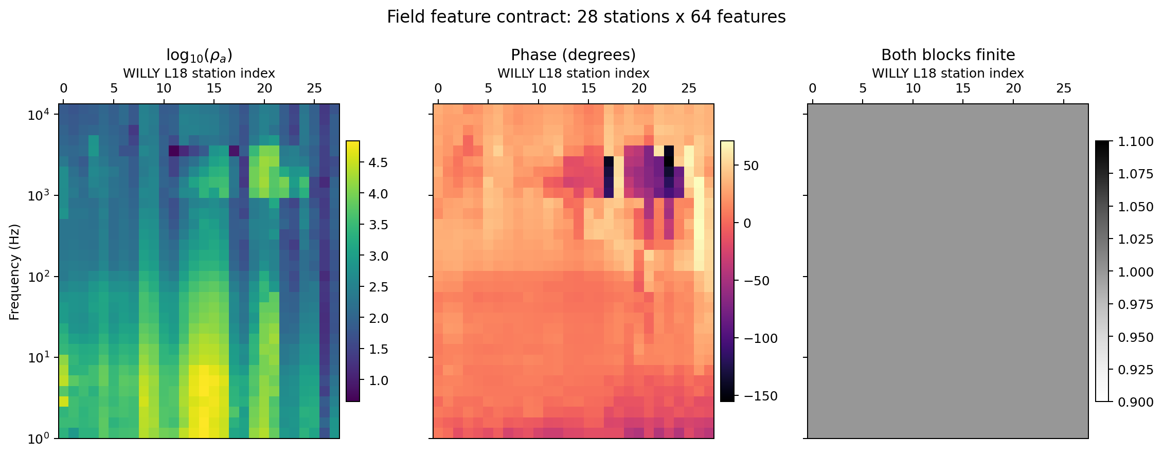
The two feature blocks in equation (1) retain frequency structure across all 28 stations. Stations are columns labelled along the top, while frequency increases vertically on the logarithmic axis. The finite-value panel is a required audit: a correctly shaped matrix can still be unusable when its requested grid extends beyond measured support.#
Warning
sites_to_features_1d leaves values outside an individual station’s
measured frequency range as nan. A neural network may reject or silently
propagate these values. Choose a common range supported by the required
stations, define a documented mask/imputation policy, and reproduce that
policy in synthetic training data.
pycsamt.ai.inversion.obs_to_features_1d() accepts already extracted
observations. In the current implementation it fills missing log resistivity
with 2.0 and missing phase with 45.0. Those constants correspond to
100 ohm metres and 45 degrees, not a neutral missing-value representation.
Use this convenience only when that policy is part of the trained contract;
otherwise handle masks explicitly in a controlled preprocessing step.
Record the contract as machine-readable metadata:
representation: mt_rho_phase_1d
component: xy
frequency_unit: Hz
frequency_order: low_to_high
n_frequencies: 32
frequency_min: 1.01
frequency_max: 10000.0
feature_layout: [log10_rho_block, phase_deg_block]
missing_policy: explicit_mask_and_training_median
6.3.12.6. 5. Build a 2-D field panel#
pycsamt.ai.inversion.sites_to_panel_2d() produces a batch containing one
field profile:
>>> from pycsamt.ai.inversion import sites_to_panel_2d

>>> X_profile, frequencies_hz, station_names = sites_to_panel_2d(
...     sites,
...     n_freqs=32,
...     n_components=4,
...     comp_te="xy",
...     comp_tm="yx",
...     freq_min=1.01,
...     freq_max=1e4,
... )

>>> print(X_profile.shape)
(1, 4, 32, 28)
For four channels, the order is:
[log10(rho_TE), phase_TE, log10(rho_TM), phase_TM]
For two channels, only TE log resistivity and phase are included. The returned panel frequency axis is high to low.
The bridge preserves input station order; it does not infer profile order from coordinates. Sort the source survey by reviewed chainage before panel creation, and preserve a station-name-to-column table. If the network requires a fixed station count, document padding, cropping, resampling, and masks.
Inspect missingness by channel and station:
>>> import numpy as np

>>> missing_fraction = np.mean(~np.isfinite(X_profile), axis=(0, 1, 2))
>>> print(missing_fraction.shape)
(28,)
>>> for name, fraction in list(zip(station_names, missing_fraction))[:4]:
...     print(name, round(float(fraction), 3))
18-001A 0.0
18-002U 0.0
18-003A 0.0
18-004A 0.0
Do not fill all missing values with a smooth interpolation unless training contains the same pattern. Interpolation can manufacture lateral continuity.
6.3.12.7. 6. Prepare coordinates for graph inversion#
pycsamt.ai.inversion.sites_to_coords_3d() returns station coordinates in
metres:
>>> from pycsamt.ai.inversion import sites_to_coords_3d

>>> coords_m = sites_to_coords_3d(
...     sites,
...     station_spacing=500.0,
... )
>>> print(coords_m.shape)
(28, 2)
>>> print(coords_m[:3])
[[    8.19238802 -1300.78745238]
 [   14.47695964 -1208.02078571]
 [    9.76353092 -1102.26678571]]
The helper attempts a local flat-earth conversion from site latitude and
longitude. When coordinates are absent or do not span a meaningful range, it
falls back to a uniformly spaced layout using station_spacing.
For production graph inversion, prefer authoritative projected coordinates and pass them explicitly to the inverter or agent. A fallback line can make an areal survey look regular and change graph connectivity without an obvious error. Verify:
coordinate units are metres;
axes have the intended orientation;
order matches feature rows and station names;
duplicate coordinates are resolved;
inter-station distances are plausible;
CRS and projection are recorded;
adjacency does not cross known structural barriers unintentionally.
6.3.12.8. 7. Design synthetic earth models#
Synthetic models should cover plausible geology without becoming physically meaningless. Define distributions for:
number of layers;
linear resistivity in ohm metres;
layer thickness and total depth;
correlations between lithology, resistivity, and thickness;
conductive and resistive targets;
weathering and basement structures;
lateral correlation lengths for spatial surveys;
rare but decision-critical cases;
nuisance parameters not intended as prediction targets.
Broad independent uniform sampling is not automatically conservative. It can overrepresent impossible combinations and underrepresent coherent geological sequences. Use scenario-aware generators where justified, and preserve the scenario label so performance can be reported by geology rather than only as one aggregate metric.
Target transformations#
The 1-D generator uses LayeredModel.to_vector(log_rho=True). The target
contains log10 resistivities followed by interface thicknesses according to
the current model-vector contract. Inspect the generated target and inverter
configuration rather than assuming all target blocks use the same scaling.
For a fixed \(L\)-layer target, a common supervised target is
In equation (2), \(\rho_\ell\) is resistivity
in ohm metres and \(h_\ell\) is the finite layer thickness in metres. If
log_thickness=True is used later
by an inverter, record whether thickness was transformed during dataset
generation, target preprocessing, or model training; mixing those locations is
an easy way to make a checkpoint unreproducible.
Variable layer counts produce vectors of different length; the batch generator
pads shorter targets with nan to the largest parameter length. Not every
network or loss can train safely on NaN targets. Use a fixed layer count for a
fixed-output inverter, or implement and test an explicit mask-aware target
strategy.
6.3.12.9. 8. Generate a 1-D synthetic dataset#
pycsamt.forward.batch.generate_dataset() supports "mt1d",
"csamt1d", and "tem1d":
>>> import numpy as np
>>> from pycsamt.forward.batch import generate_dataset

>>> frequencies_hz = np.logspace(np.log10(1.01), 4, 32)

>>> dataset = generate_dataset(
...     solver="mt1d",
...     n_samples=40,
...     freqs=frequencies_hz,
...     n_layers=5,
...     rho_range=(1.0, 10_000.0),
...     depth_max=2000.0,
...     noise_level=0.05,
...     noise_type="field",
...     include_phase=True,
...     seed=42,
...     n_jobs=1,
...     output=None,
...     verbose=False,
... )

>>> print(dataset)
ForwardDataset(n=40, n_features=64, n_params=9, solver='mt1d')
>>> print(dataset.X.shape)
(40, 64)
>>> print(dataset.y.shape)
(40, 9)
For MT with phase, X contains a log10 apparent-resistivity block followed
by a phase block. For TEM, it contains log10 absolute decay values. Confirm the
feature size from the generated array rather than hard-coding it in downstream
code.
Generator parameters#
solverForward method. It must match the field method and feature contract.
n_samplesNumber of synthetic examples. The small value above keeps the documentation example quick; adequacy in a real run depends on parameter dimension, distribution complexity, architecture, and rare-case coverage.
n_layersFixed integer or inclusive
(low, high)range. Fixed-output supervised models are simplest with a fixed value.rho_rangeLinear resistivity bounds in ohm metres used by random model generation.
depth_maxMaximum synthetic model depth in metres.
noise_levelandnoise_typeRelative noise magnitude and one of
"gaussian","multiplicative", or"field".geologyOptional named scenario forwarded to
LayeredModel.from_geology. Validate available scenario names in the installed implementation.seedBase seed from which deterministic worker seeds are drawn.
n_jobsWorker process count;
-1uses available CPU cores. Parallel completion order can affect row order, so do not assume sample index maps directly to generation seed unless explicitly recorded and verified.outputOptional compressed NPZ destination.
TEM generation uses numerical integration and can be substantially slower. Pilot the physics and storage requirements before launching a large dataset.
6.3.12.10. 9. Understand ForwardDataset#
pycsamt.forward.batch.ForwardDataset stores:
XFeature matrix
(n_samples, n_features).yTarget matrix
(n_samples, n_parameters).freqsortimesSampling grid used by the forward responses.
metaIn-memory structured metadata containing layer count and noise level in the current generator.
solverSolver identifier.
Save and load without pickle:
>>> from pycsamt.forward.batch import ForwardDataset

>>> dataset.save("datasets/mt1d_5layer.npz")
>>> restored = ForwardDataset.load("datasets/mt1d_5layer.npz")
>>> print(restored)
ForwardDataset(n=40, n_features=64, n_params=9, solver='mt1d')
The current NPZ serialization preserves arrays, solver, frequency/time grids, and metadata fields for layer count and noise level. It does not preserve the complete generator configuration such as resistivity range, depth limit, noise type, geology, job count, or base seed. Store those in a companion JSON or YAML manifest.
6.3.12.11. 10. Generate pseudo-3-D graph data#
pycsamt.forward.batch.generate_dataset_3d() creates spatially correlated
layered station models for pycsamt.ai.inversion.GCNInverter3D:
>>> from pycsamt.forward.batch import generate_dataset_3d

>>> surveys = generate_dataset_3d(
...     solver="mt1d",
...     n_surveys=20,
...     n_stations=25,
...     n_layers=5,
...     freqs=frequencies_hz,
...     extent=10_000.0,
...     corr_length=2000.0,
...     log_rho_mean=2.0,
...     log_rho_std=0.6,
...     thickness_range=(100.0, 1500.0),
...     station_layout="grid",
...     noise_level=0.03,
...     noise_type="field",
...     include_phase=True,
...     seed=42,
...     n_jobs=1,
...     output=None,
...     verbose=False,
... )

>>> print(surveys.X.shape)
(20, 25, 64)
>>> print(surveys.y.shape)
(20, 25, 9)
>>> print(surveys.coords.shape)
(25, 2)
The small n_surveys value above is for documentation speed; production
graph training usually needs many more survey realizations. The generator
currently uses the MT 1-D forward solver at every graph node.
Per-layer log resistivities are drawn from a spatially correlated Gaussian
random field. Layer thicknesses are log-uniform and spatially constant within
one synthetic survey. All surveys share one station layout.
This is a pseudo-3-D graph-training distribution, not a full 3-D EM forward simulation. Its correlation length and flat-layer assumptions strongly affect what spatial patterns the graph network learns.
pycsamt.forward.batch.SurveyDataset3D saves, loads, and splits along
the survey axis. Its NPZ metadata retains correlation length and noise level,
but the full generator configuration still requires a companion manifest.
6.3.12.12. 11. Prepare 2-D training profiles#
The current package has two deliberately distinct ways to prepare a profile
inverter. Tiling or correlating station-wise 1-D responses remains the cheap
pseudo-2-D training model used by the default Inv2DAgent path. For
lateral electromagnetic coupling,
pycsamt.ai.training.dataset2d.generate_2d_maxwell_dataset() now generates
2-D Maxwell training model realizations with the verified
pycsamt.forward.maxwell.mt2d.MT2DAdapter.
The Maxwell route begins from one shared pycsamt.ai.geology.GeologyGrid.
For realization \(r\), a seeded standardized Gaussian field
\(g_r(z,x)\) is converted to resistivity by
where the horizontal and vertical correlation lengths are independently drawn from the configured ranges. Equation (3) is a statistical field prior, not a lithological model: it produces smooth, correlated heterogeneity but does not create faults, contacts, or facies unless those structures are supplied by a different geological generator.
A small fully executed example is:
>>> from pycsamt.ai.geology import GeologyGrid
>>> from pycsamt.ai.training.dataset2d import (
...     Maxwell2DDatasetConfig,
...     generate_2d_maxwell_dataset,
... )

>>> grid = GeologyGrid.regular_2d(
...     nx=6, nz=4, dx_m=300.0, dz_m=150.0
... )
>>> config = Maxwell2DDatasetConfig(
...     dataset_id="guide-2d-v1",
...     grid=grid,
...     correlation_length_x_m=(600.0, 900.0),
...     correlation_length_z_m=(150.0, 300.0),
...     frequencies_hz=[10.0, 3.0],
...     station_x_m=[600.0, 900.0, 1200.0],
...     n_realizations=2,
...     seed=0,
...     validation_fraction=0.0,
...     test_fraction=0.0,
... )
>>> maxwell_2d = generate_2d_maxwell_dataset(config)
>>> first_2d = maxwell_2d.samples[0]
>>> len(maxwell_2d.samples), maxwell_2d.rejected
(2, ())
>>> first_2d.resistivity_ohm_m.shape, first_2d.survey.shape
((4, 6), (3, 2, 2))
>>> first_2d.survey.components
('zxy', 'zyx')
>>> first_2d.mesh_cells, f"{first_2d.relative_residual:.3e}"
(8650, '2.290e-17')
>>> maxwell_2d.split.sizes
{'train': 2, 'validation': 0, 'test': 0}
>>> maxwell_2d.manifest.dataset_id, maxwell_2d.manifest.sample_count
('guide-2d-v1', 2)
>>> len(maxwell_2d.manifest.configuration_hash)
64
The target has shape (depth, x)=(4, 6) on the geological grid. The input
is a canonical SurveyData with shape
(station, frequency, component)=(3, 2, 2); its component order is the
requested TE zxy followed by TM zyx. A U-Net adapter must explicitly
convert each complex impedance to its declared channels and transpose the
batch to (realization, channel, frequency, station). A compatible target
batch is (realization, depth, x). Never infer these transformations merely
from equal axis lengths.
Each finite-difference solve records the linear-system solver residual
and the sample stores the maximum over simulated frequencies. The
\(2.290\times10^{-17}\) value above shows that the discrete linear systems
were solved accurately; it does not establish mesh convergence, correct
boundary placement, or geological realism. Those require half-space and
layered benchmarks plus grid-refinement tests. The mesh uses uniform lateral
spacing and a continuously graded depth progression, with its extent tied to
skin depth and mesh_safety_factor. max_mesh_cells raises before an
intractably wide uniform mesh is launched rather than silently coarsening it.
Only converged results become samples. Failed or non-converged realization IDs
are retained in rejected; if every realization fails, generation raises
instead of returning an empty training set. A rejection policy is part
of the distribution because solver failures can cluster around conductive,
resistive, or geometrically difficult cases. Report rejection rate and target
statistics for rejected attempts so the accepted corpus is not mistaken for
the originally requested prior.
The example disables validation and test partitions only to keep two attempted
solves meaningful. A real corpus must request enough independent realizations
for non-empty, realization-level splits. The generated
DatasetManifest records the complete config
and split, while an optional MaxwellResultCache
makes problem-hash-identical solves resumable. Cache reuse changes execution
cost, not the required manifest or acceptance checks.
These responses are deliberately clean and noiseless. Apply field-matched
dropout, static shift, distortion, and noise afterward with
pycsamt.ai.domain_gap.simulator, preserving the clean realization ID as
lineage so its corrupted variants cannot leak across dataset partitions.
Topography is also not implicit: this generator places receivers on the flat
surface of the configured grid. A field workflow that claims terrain-aware
physics needs a solver mesh and receiver geometry that encode terrain, not a
post-hoc drape of the target image.
6.3.12.13. 12. Prepare 3-D training profiles#
Section 10’s pseudo-3-D graph data and AI inversion agents’s default
Inv3DAgent(physics="mt1d") both still tile independent 1-D columns
under a graph-smoothing network; nothing in that training data ever shows
the network a laterally and vertically coupled response. For
Genuine 3-D Maxwell training,
pycsamt.ai.training.dataset3d.generate_3d_maxwell_dataset() generates
correlated 3-D resistivity volumes and solves each one with the
research-only pycsamt.forward.maxwell.mt3d.MT3DAdapter, the same
role generate_2d_maxwell_dataset()
plays for profile data. Inv3DAgent(physics="mt3d") is the agent that
consumes it.
The same log-resistivity construction as equation
(3) applies unchanged with a third spatial
argument, \(\rho_r(z,y,x)=10^{\mu_{\log\rho}+\sigma_{\log\rho}g_r(z,y,x)}\),
once the correlated field itself is drawn from a 3-D
GaussianCorrelation supplying length_y_m.
A larger n_realizations explores more draws from this prior; it does not
turn the prior into faults, lenses, stratigraphic contacts, or facies. Those
geometries require a different generator and must remain distinguishable in
the manifest so that split and coverage audits can be performed by geological
family.
Preparation uses three related grids. Let \(G_g\) denote the geological grid, \(G_s\) the padded solver mesh, and \(G_o\) the agent’s output grid. A piecewise-constant operator \(P_{g\rightarrow s}\) transfers conductivity into the cells used by the Maxwell solve,
The first mapping extends the nearest geological edge cell into the padding; the second samples each station’s true vertical column onto the requested display depths. Consequently, equal array sizes do not make these grids interchangeable. Record their edges, axis order, coordinate reference, units, and both mappings with the dataset.
A small fully executed example, matching section 11’s scale:
>>> from pycsamt.ai.geology import GeologyGrid
>>> from pycsamt.ai.training.dataset3d import (
...     Maxwell3DDatasetConfig,
...     generate_3d_maxwell_dataset,
... )

>>> grid3 = GeologyGrid.regular_3d(
...     nx=4, ny=4, nz=6, dx_m=200.0, dy_m=200.0, dz_m=100.0
... )
>>> config3 = Maxwell3DDatasetConfig(
...     dataset_id="guide-3d-v1",
...     grid=grid3,
...     correlation_length_x_m=(400.0, 800.0),
...     correlation_length_y_m=(400.0, 800.0),
...     correlation_length_z_m=(100.0, 200.0),
...     frequencies_hz=[50.0, 20.0],
...     station_xy_m=[[400.0, 400.0], [600.0, 600.0]],
...     n_realizations=2,
...     seed=0,
...     validation_fraction=0.0,
...     test_fraction=0.0,
... )
>>> maxwell_3d = generate_3d_maxwell_dataset(config3)
>>> first_3d = maxwell_3d.samples[0]
>>> len(maxwell_3d.samples), maxwell_3d.rejected
(2, ())
>>> first_3d.resistivity_ohm_m.shape, first_3d.survey.shape
((6, 4, 4), (2, 2, 2))
>>> first_3d.survey.components
('zxy', 'zyx')
>>> first_3d.mesh_cells, f"{first_3d.relative_residual:.3e}"
(3584, '2.197e-19')
>>> maxwell_3d.split.sizes
{'train': 2, 'validation': 0, 'test': 0}
>>> maxwell_3d.manifest.dataset_id, maxwell_3d.manifest.sample_count
('guide-3d-v1', 2)
>>> len(maxwell_3d.manifest.configuration_hash)
64
The target is a volume of shape (z, y, x)=(6, 4, 4) on the geological
grid, not a profile section. GCNInverter3D does not consume it as a
dense image the way a U-Net consumes section 11’s 2-D target: each real
station’s true vertical resistivity column is resampled out of the volume
at that station’s own (x, y) position onto the agent’s display depth
grid, so the geological grid’s own resolution need not match the number of
output layers. Equation (4) – the linear
solver residual – applies unchanged to this solve; the
\(2.197\times10^{-19}\) value above again shows an accurate linear
solve, not mesh convergence or geological realism.
The receiver contract is equally strict. station_xy_m contains
(x, y) coordinates in metres inside the geological grid, and the current
generator evaluates them at the flat surface \(z=0\). Elevations may be
retained for display and graph geometry, but neither MT3DAdapter nor the
current ModEm3DAdapter configuration turns those elevations into active
terrain cells. A terrain-aware claim therefore requires a separately
validated mesh and receiver workflow; draping a section afterward changes
the visualization, not the forward physics.
Unlike section 11’s uniform lateral mesh, the 3-D solver mesh is padded
and non-uniform, because 3-D cell count scales as the cube of resolution
rather than its square – a uniform mesh both fine enough for the
structure and extensive enough for skin depth in three directions
at once rarely fits max_mesh_cells. See 3-D Maxwell training-data generation for the full
mesh construction, the cells_per_skin_depth frequency-aware core
resolution knob, and its own realization-gallery and full-tensor-response
figures – this section deliberately does not repeat them. As with the
2-D route, only converged realizations become samples,
rejected records
the rest, and pycsamt.ai.domain_gap.simulator’s noise, dropout, and
distortion apply identically afterward, since it operates on the shared
SurveyData contract without any notion
of how many spatial dimensions produced it.
cells_per_skin_depth defaults to None, which preserves the geological
grid’s native core spacing. Set it explicitly only after choosing a frequency
band and a cell budget; for example, 8.0 requests eight core cells across
the shallowest skin depth, capped at the geological-grid spacing. The bundled
small-grid benchmark is calibrated most strongly at frequencies up to 2 Hz.
At tens of hertz, verify half-space error and mesh refinement for the actual
resistivity range instead of treating a small linear-system residual as an
accuracy certificate.
The dataset generator is intentionally wired to the pure-Python
MT3DAdapter so small reproducible tests
do not depend on an external executable. This is not the same backend as
ModEm3DAdapter. For a production
corpus, build the same solver-neutral Maxwell problems, run the compiled
ModEM adapter, assess every result, and convert accepted responses back to the
same SurveyData and target contracts. Do not label a corpus as ModEM
generated merely because physics="mt3d" was selected in the agent: that
agent path currently invokes MT3DAdapter.
A genuine 3-D solve costs far more per realization than a 2-D one –
seconds to tens of seconds even at this documentation scale, against a
2-D realization’s fraction of a second – so budget n_realizations
deliberately rather than reusing a 2-D-sized default, and prefer
MaxwellResultCache so an interrupted
generation run resumes instead of restarting. Preserve the cache beside the
manifest, accepted realization IDs, rejected attempts and reasons, exact
split indices, and normalization arrays. If difficult conductivity fields
fail more often, the accepted set is a different distribution; replacing
failures with fresh draws without recording them hides that bias.
6.3.12.14. 13. Add realistic observation effects#
White Gaussian noise alone rarely represents field data. Consider controlled augmentation for:
frequency-dependent and component-dependent errors;
multiplicative apparent-resistivity noise;
phase noise;
missing frequencies and bands;
station dropout;
outliers and spikes;
static shifts;
smooth calibration bias;
source and near-field effects for controlled-source data;
coordinate perturbations for graph workflows;
preprocessing alternatives used by the field pipeline.
Separate effects the model should become robust to from effects that should
trigger rejection. If training always imputes a missing band, the model may
produce a confident prediction where the operational policy should instead
return needs_review.
Do not augment validation and test sets by copying training examples with new noise. That tests denoising around known models rather than generalization to new earth structures.
6.3.12.15. 14. Audit synthetic arrays#
Run structural and numerical checks immediately after generation:
>>> import numpy as np

>>> assert dataset.X.ndim == 2
>>> assert dataset.y.ndim == 2
>>> assert len(dataset.X) == len(dataset.y)
>>> assert np.all(np.isfinite(dataset.X))

>>> target_finite = np.isfinite(dataset.y)
>>> print("Target finite fraction:", target_finite.mean())
Target finite fraction: 1.0
>>> print(
...     "Feature percentiles:",
...     np.round(np.nanpercentile(dataset.X, [0, 1, 50, 99, 100]), 3),
... )
Feature percentiles: [-0.098  0.317 10.157 84.282 96.21 ]
>>> print(
...     "Target percentiles:",
...     np.round(np.nanpercentile(dataset.y, [0, 1, 50, 99, 100]), 3),
... )
Target percentiles: [4.700000e-02 1.370000e-01 3.660000e+00 1.364546e+03 1.710847e+03]
Also inspect:
samples at parameter bounds;
layer-count balance;
depth and thickness distributions;
response curves from randomly selected models;
correlations among target parameters;
frequency-wise means and spreads;
phase wrapping or implausible values;
effects of each noise model;
duplicated examples;
generator failures and rejected cases.
Plot distributions by split and scenario. Aggregate percentiles can hide a missing rare target class.
6.3.12.16. 15. Split without leakage#
ForwardDataset.split provides a random row split:
>>> train, validation, test = dataset.split(
...     val_frac=0.15,
...     test_frac=0.15,
...     seed=42,
... )
>>> print(len(train), len(validation), len(test))
28 6 6
>>> print(train.X.shape, validation.X.shape, test.X.shape)
(28, 64) (6, 64) (6, 64)
This is appropriate only when rows are independent and exchangeable. It does not enforce grouping by geological scenario, parent model, augmentation family, or generation batch.
Prefer group-based splitting when examples are related:
keep all noise realizations of one earth model in one split;
keep correlated profiles from one geological realization together;
split graph data by survey, not station;
hold out complete geology scenarios to test extrapolation;
reserve a calibration set distinct from validation and test;
freeze split indices before architecture selection.
SurveyDataset3D.split correctly splits along the synthetic survey axis,
but scenario-aware grouping may still require custom indices.
For 2-D Maxwell data, use the dataset’s existing RealizationSplit rather
than applying ForwardDataset.split to converted U-Net rows. If one clean
realization later produces several noise or dropout variants, bind all of them
to the clean realization ID and regenerate a lineage-aware split as documented
in Canonical data contracts.
Never choose hyperparameters on the test set. Once a test result changes model or data preparation decisions, that set has become validation data.
6.3.12.17. 16. Fit preprocessing on training only#
If features or targets are standardized, compute statistics from the training set only:
The index \(j\) identifies one fixed frequency-channel feature. Equation (6) must use the same saved \(\mu_j\) and \(\sigma_j\) for validation, test, calibration, and WILLY field rows; estimating them again on any of those sets changes the transformation.
>>> x_mean = np.nanmean(train.X, axis=0)
>>> x_std = np.nanstd(train.X, axis=0)
>>> x_std = np.where(x_std > 0, x_std, 1.0)

>>> X_train_scaled = (train.X - x_mean) / x_std
>>> X_val_scaled = (validation.X - x_mean) / x_std
>>> X_test_scaled = (test.X - x_mean) / x_std
>>> X_field_scaled = (X_field - x_mean) / x_std
>>> print(
...     X_train_scaled.shape,
...     X_val_scaled.shape,
...     X_test_scaled.shape,
...     X_field_scaled.shape,
... )
(28, 64) (6, 64) (6, 64) (28, 64)
This example does not resolve NaNs; apply the documented mask or imputation policy first or within a pipeline designed for missing values.
Save normalization arrays with the checkpoint. Recomputing them from field data changes the model and leaks the deployment distribution into inference.
For target scaling, preserve inverse-transform code and units. Validate that a round trip returns the original target within numerical tolerance.
6.3.12.18. 17. Compare field and synthetic domains#
Before training acceptance or field inference, compare X_field with
training data:
>>> train_low = np.nanpercentile(train.X, 1, axis=0)
>>> train_high = np.nanpercentile(train.X, 99, axis=0)

>>> outside = (X_field < train_low) | (X_field > train_high)
>>> outside_fraction = np.nanmean(outside, axis=1)

>>> for name, fraction in list(zip(station_names, outside_fraction))[:4]:
...     print(name, round(float(fraction), 3))
18-001A 0.688
18-002U 0.703
18-003A 0.703
18-004A 0.719
This per-feature envelope is only a basic diagnostic. It ignores feature correlation and does not prove in-distribution status; with only 40 synthetic examples it is intentionally a smoke test, not acceptance evidence. Add multivariate or latent-distance diagnostics where appropriate.
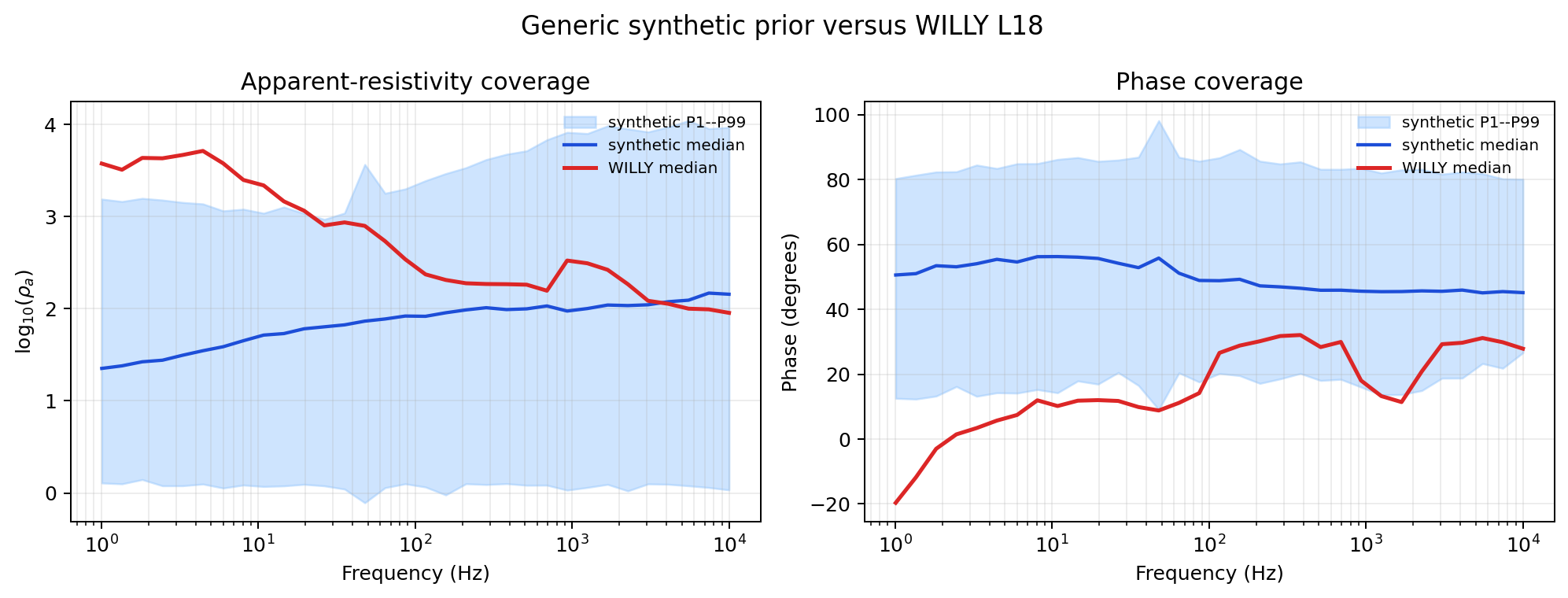
Much of the WILLY median response lies outside the central synthetic envelope generated by the deliberately small, generic model prior. The mismatch is evidence to redesign the prior and nuisance effects before training; it is not evidence that the field curve is erroneous.#
Review domain coverage by:
station and frequency;
component and feature type;
missingness pattern;
response-curve shape;
survey geometry and adjacency degree;
known geology and nuisance effects;
acquisition and processing version.
Define operational thresholds before reviewing target predictions. Stations outside the supported domain should be flagged, withheld, or handled by a separate validated model—not silently extrapolated.
6.3.12.19. 18. Store datasets with provenance#
A useful dataset record is:
datasets/mt1d_5layer_v001/
├── dataset.npz
├── manifest.yml
├── generation_config.yml
├── feature_contract.yml
├── split_indices.npz
├── normalization.npz
├── checksums.sha256
├── audit/
│   ├── distributions.csv
│   ├── coverage_by_scenario.csv
│   └── rejected_samples.csv
└── figures/
    ├── parameter_distributions.png
    ├── response_envelopes.png
    └── field_coverage.png
The manifest should include:
stable dataset ID and revision;
generator code/version and configuration;
solver and physics assumptions;
feature and target schemas with units;
sample count and rejection count;
base and worker-seed policy;
field/QC source identifiers;
split method and exact indices;
preprocessing and normalization values;
file hashes;
limitations and intended use;
author, reviewer, status, and date.
Compressed NPZ is convenient for trusted numeric arrays. Do not enable pickle for untrusted datasets. Treat checkpoints, datasets, and manifests as a linked versioned set.
6.3.12.20. Complete 1-D preparation example#
>>> from pathlib import Path
>>> import json
>>> import numpy as np

>>> from pycsamt.ai.inversion import sites_to_features_1d
>>> from pycsamt.emtools._core import ensure_sites
>>> from pycsamt.forward.batch import generate_dataset

>>> root = Path("datasets/mt1d_5layer_v001")
>>> root.mkdir(parents=True, exist_ok=True)

>>> frequencies_hz = np.logspace(np.log10(1.01), 4, 32)

>>> dataset = generate_dataset(
...     solver="mt1d",
...     n_samples=40,
...     freqs=frequencies_hz,
...     n_layers=5,
...     rho_range=(1.0, 10_000.0),
...     depth_max=2000.0,
...     noise_level=0.05,
...     noise_type="field",
...     include_phase=True,
...     seed=42,
...     n_jobs=1,
...     verbose=False,
... )
>>> dataset.save(root / "dataset.npz")

>>> train, validation, test = dataset.split(
...     val_frac=0.15,
...     test_frac=0.15,
...     seed=42,
... )
>>> train.save(root / "train.npz")
>>> validation.save(root / "validation.npz")
>>> test.save(root / "test.npz")

>>> sites = ensure_sites(
...     "data/AMT/WILLY_data/L18PLT",
...     recursive=True,
...     verbose=0,
... )
>>> X_field, field_freqs, station_names = sites_to_features_1d(
...     sites,
...     comp="xy",
...     n_freqs=32,
...     freq_min=float(frequencies_hz.min()),
...     freq_max=float(frequencies_hz.max()),
... )

>>> if not np.allclose(field_freqs, frequencies_hz):
...     raise ValueError("Synthetic and field frequency grids differ.")

>>> np.savez_compressed(
...     root / "field_features.npz",
...     X=X_field,
...     freqs=field_freqs,
...     station_names=np.asarray(station_names),
... )

>>> manifest = {
...     "dataset_id": "mt1d_5layer_v001",
...     "solver": "mt1d",
...     "n_samples": 40,
...     "n_layers": 5,
...     "rho_range_ohm_m": [1.0, 10_000.0],
...     "depth_max_m": 2000.0,
...     "noise_type": "field",
...     "noise_level": 0.05,
...     "seed": 42,
...     "component": "xy",
...     "feature_layout": "log10_rho_block_then_phase_deg_block",
... }
>>> (root / "manifest.json").write_text(
...     json.dumps(manifest, indent=2),
...     encoding="utf-8",
... )
339
>>> print(dataset)
ForwardDataset(n=40, n_features=64, n_params=9, solver='mt1d')
>>> print(train.X.shape, validation.X.shape, test.X.shape)
(28, 64) (6, 64) (6, 64)
>>> print(X_field.shape, len(station_names))
(28, 64) 28
>>> print(sorted(p.name for p in root.iterdir()))
['dataset.npz', 'field_features.npz', 'manifest.json', 'test.npz', 'train.npz', 'validation.npz']
For a controlled project, save the exact split indices rather than only the three subset files, use a production-scale sample count, and add checksums plus field-coverage diagnostics.
6.3.12.21. Review checklist#
Check |
Required evidence |
|---|---|
Scientific target defined |
Method, dimension, parameterization, depth, units, and decision need. |
Field inputs reviewed |
Canonical load, QC, components, frequency coverage, coordinates, processing, exclusions, and station order. |
Feature contract frozen |
Transformation, order, grid, units, masks, imputation, and normalization. |
Synthetic geology defensible |
Parameter distributions, dependencies, scenarios, rare targets, and impossible-case controls. |
Forward physics documented |
Solver, dimension, geometry, approximations, and numerical settings. |
Observation effects realistic |
Noise, missingness, distortion, outliers, and rejection behavior. |
Targets train safely |
Shape, units, transformation, bounds, NaN padding, and inverse transform. |
Splits resist leakage |
Group definitions, frozen indices, calibration separation, and untouched final test set. |
Preprocessing is isolated |
Statistics fitted on training only and saved with the checkpoint. |
Field coverage established |
Per-feature, multivariate, missingness, geometry, and scenario checks. |
Dataset is reproducible |
Arrays, generator configuration, metadata, seeds, checksums, splits, audit figures, author, and version. |
6.3.12.22. Common mistakes#
Avoid these errors:
treating valid impedance loading as complete QC;
using different frequency grids for synthetic and field features;
confusing low-to-high 1-D grids with high-to-low 2-D panel axes;
ignoring NaNs created outside station frequency ranges;
accepting constant 100-ohm-m/45-degree imputation without documenting it;
assuming the 2-D bridge sorts stations by profile distance;
using coordinate fallback geometry as authoritative survey geometry;
training fixed-output networks on NaN-padded variable-layer targets without a tested mask-aware loss;
calling correlated 1-D graph examples full 3-D EM simulations;
assuming
Inv3DAgent(physics="mt3d")invokes the compiled ModEM backend, or treating the small-grid research solver as production validation;using station elevations or a draped section as evidence that topography participated in the 3-D Maxwell equations;
calling tiled 1-D profile responses 2-D Maxwell training data, or treating a small linear-system residual as evidence of mesh convergence;
discarding failed 2-D forward realizations without auditing how rejection changed the requested geological distribution;
splitting noise realizations of the same earth model across train and test;
fitting normalization on the complete dataset or field observations;
relying on NPZ alone to preserve generator provenance;
using marginal min/max coverage as proof that field inputs are in domain;
discarding failed or rejected synthetic samples without recording them.
6.3.12.23. Next steps#
Continue with:
AI model selection to select architecture and dimension for the frozen data contract;
Training AI inversion models to fit preprocessing and model parameters correctly;
AI inversion validation to evaluate leakage, response reconstruction, and domain transfer;
AI inversion inference to apply the exact field transformation at deployment;
AI inversion uncertainty to assess calibration and distribution shift;
AI inversion reporting to publish dataset and model provenance.
The two diagnostic figures on this page are reproduced by
docs/scripts/generate_ai_inversion_figures.py. They use the bundled WILLY
L18 observations; the synthetic envelope is deterministic teaching data from
seed 42, not an accepted training distribution or inversion result.