
6.3.15. AI inversion inference#
Inference applies a fitted AI inversion model to observations that were not used to update its parameters. Although the network call may take only milliseconds, a reliable inference workflow includes checkpoint verification, exact preprocessing replay, input-domain assessment, output decoding, forward response reconstruction, uncertainty, scientific review, and controlled export.
This guide assumes that the dataset and model have already passed the procedures in AI inversion data preparation, Training AI inversion models, and AI inversion validation. Inference is not the stage at which an unvalidated checkpoint becomes valid.
Compatibility before prediction
Never run a checkpoint on an array merely because its shape matches. The feature meaning, order, units, grid, normalization, target parameterization, backend, and model metadata must match the approved training contract.
6.3.15.1. Inference workflow#
identify the approved model and deployment policy;
verify checkpoint integrity and compatibility;
load and QC field observations;
reproduce the feature contract exactly;
apply saved missing-value and normalization transformations;
gate unsupported or out-of-distribution inputs;
run prediction without changing model state;
decode outputs into documented physical units;
reconstruct responses and inspect residuals;
calculate calibrated uncertainty where available;
apply acceptance, review, or rejection rules;
export predictions with station order and provenance.
6.3.15.2. 1. Define the inference unit#
The unit passed to the model depends on architecture:
- 1-D
One row per station. Stations can be batched, but each prediction is independent unless an ensemble or later spatial operation is applied.
- 2-D
One complete ordered profile panel per batch item. Station count, order, channel count, frequency grid, and depth target must match training.
- Graph 3-D
One survey graph or a batch of graphs sharing compatible node and feature conventions. Predictions depend on feature rows and adjacency together.
- PINN or hybrid
Observations are attached at construction time rather than passed to
predict(X). Both still require an explicitfit()call beforepredict()— there is no stateless, pre-fitted deployment path for these classes.
Do not split a profile or graph into convenient batches if that changes the spatial context learned by the model.
6.3.15.3. 2. Assemble the approved model package#
An inference package should contain:
checkpoint or fitted-model artifact;
checksum and model identifier;
architecture and backend information;
feature schema and exact frequency/time grid;
saved normalization or preprocessing state;
output schema, transformations, and units;
training-distribution summary;
validation and calibration metrics;
intended methods, geometry, and operating domain;
known failure modes and rejection thresholds;
software and dependency versions;
approval status and reviewer.
A standalone weights file is insufficient. If the feature contract cannot be reconstructed unambiguously, the checkpoint should not be deployed.
6.3.15.4. 3. Verify integrity and compatibility#
Before loading, verify the artifact checksum using the project’s approved integrity tooling. Then compare model metadata with the inference request:
Compatibility field |
Required match |
|---|---|
Method and solver |
MT, CSAMT, TEM, or other documented physics and response convention; for learned 3-D models, preserve the training forward backend separately from the deep-learning runtime backend. |
Parameterization |
Layer count, depth grid, thickness representation, and output order. |
Features |
Components, apparent resistivity/phase or impedance channels, block order, transformations, and masks. |
Sampling grid |
Exact frequencies or times, order, unit, and interpolation rule. |
Normalization |
Saved training statistics and transformation version. |
Geometry |
Station count/order for 2-D; coordinates and graph policy for 3-D. |
Backend |
Compatible PyTorch/TensorFlow model construction and weight format. |
Operating domain |
Supported ranges, noise, missingness, geology, and survey layout. |
Reject incompatibility rather than modifying field arrays until the model runs. Any deliberate adapter becomes a new preprocessing version that requires validation.
6.3.15.5. 4. Load a 1-D checkpoint#
pycsamt.ai.inversion.EMInverter1D explicitly saves weights,
normalizers, hyperparameters, history, and selected metadata:
>>> from pathlib import Path
>>> from pycsamt.ai.inversion import EMInverter1D
>>> checkpoint = Path("checkpoints/mt1d_resnet_5layer.npz")
>>> inverter = EMInverter1D.load(checkpoint)
>>> inverter.n_layers, inverter.arch, inverter.log_thickness
(5, 'resnet', True)
Loading restores the backend recorded in the checkpoint and rebuilds the network. The compatible deep-learning backend must be installed. Treat a checkpoint as executable model content and load only trusted artifacts. This particular checkpoint was trained on the Willy AMT line’s own frequency band — 32 log-spaced frequencies from 1.05 to 9500 Hz — which matters for every example that follows: the field feature grid must reproduce that exact band, not a value copied from a different survey or a different guide page.
Note
The named approved checkpoint and its training-percentile arrays are reference-run artifacts, not files distributed with the source checkout. The recorded outputs and existing figures below may therefore be read as a case study, but reproducing prediction values requires the reviewed model package. WILLY loading, feature-grid, finiteness, and geometry checks use bundled data and are executable directly.
Registry checkpoints can be requested with:
>>> inverter = EMInverter1D.from_pretrained(
...     "mt1d-resnet-5layer-v1",
...     cache_dir="model_cache",
... )
Registry presence does not guarantee that weights are currently downloadable
— see AI inversion agents’s ModelZooAgent walkthrough for
what a not-yet-released registry entry looks like in practice. Preserve
registry metadata and the downloaded file checksum. Do not replace a failed
download with new training while continuing to label the result as the
registry model.
6.3.15.6. 5. Prepare 1-D field features#
Use the public bridge and the checkpoint’s exact grid:
>>> from pycsamt.ai.inversion import sites_to_features_1d
>>> from pycsamt.emtools._core import ensure_sites
>>> sites = ensure_sites(
...     "data/AMT/WILLY_data/L18PLT",
...     recursive=True,
...     verbose=0,
... )
>>> X_field, frequencies_hz, station_names = sites_to_features_1d(
...     sites,
...     comp="xy",
...     n_freqs=32,
...     freq_min=1.05,
...     freq_max=9500.0,
... )
>>> X_field.shape
(28, 64)
The bridge returns the block layout [log10(rho_a), phase_deg]. Frequency
endpoints and n_freqs must come from model metadata, not memory or a
nearby example — and the boundary matters literally: these 28 stations cover
1.008–10400 Hz, so a query grid starting at freq_min=1.0 puts one point
just outside every station’s real range and returns nan there, while
freq_min=1.05 stays safely inside it.
Check the matrix before prediction:
>>> import numpy as np
>>> print("Feature shape:", X_field.shape)
Feature shape: (28, 64)
>>> print("Non-finite fraction:", np.round(np.mean(~np.isfinite(X_field), axis=1), 3))
Non-finite fraction: [0. 0. 0. 0. 0. 0. 0. 0. 0. 0. 0. 0. 0. 0. 0. 0. 0. 0. 0. 0. 0. 0. 0. 0.
 0. 0. 0. 0.]
sites_to_features_1d leaves values outside a station’s observed range as
nan. That is not a hypothetical edge case: requesting the wider band used
elsewhere in this guide series (\(10^{-4}\) to \(10^{3}\)Hz, the
AIInversionAgent default) against these same 28
stations leaves 56.25% of every feature row non-finite, because natural-source
AMT simply has no usable signal down at \(10^{-4}\)Hz. Apply only the
imputation/mask policy fitted and validated with the checkpoint — the
inverter’s stored normalizer does not define a missing-value policy by
itself, and a plain feed-forward network propagates a single nan input
into an entirely nan output rather than silently ignoring it.
6.3.15.7. 6. Replay preprocessing exactly#
For EMInverter1D, predict() applies the
normalizer restored from the fitted object. Therefore supply features in the
same pre-normalized representation used by training. Do not normalize them a
second time.
For custom models, distinguish:
- Raw transformation
Conversion from physical observations into log resistivity, phase, masks, or other feature channels.
- Grid transformation
Sorting and interpolation onto the approved frequency/time/station axes.
- Missing-value transformation
Masking or imputation using the trained policy.
- Statistical transformation
Scaling with training-only means, standard deviations, or other fitted parameters.
- Model input adaptation
Batch and channel dimensions expected by the selected backend.
Version this pipeline as one unit. A change to any stage creates a new deployment configuration and may invalidate prior validation.
6.3.15.8. 7. Gate out-of-domain inputs#
Run domain checks before predictions are visible to the interpreter. At minimum, compare each field row against training feature percentiles:
where \(P\) is feature count and the quantiles are fitted on training data only. A threshold such as \(g_s>0.10\) is an operational review rule, not the probability that station \(s\) is wrong.
>>> train_low = np.load("model_package/training_p01.npy")
>>> train_high = np.load("model_package/training_p99.npy")
>>> outside = (X_field < train_low) | (X_field > train_high)
>>> outside_fraction = np.nanmean(outside, axis=1)
>>> review_mask = outside_fraction > 0.10
>>> int(review_mask.sum())
27
The plotting code is intentionally explicit so the threshold and review classification remain visible when this diagnostic is adapted:
>>> import matplotlib.pyplot as plt
>>> fig, ax = plt.subplots(figsize=(10.5, 4.2))
>>> colors = np.where(review_mask, "#dc2626", "#16a34a")
>>> _ = ax.bar(np.arange(len(station_names)), outside_fraction, color=colors)
>>> _ = ax.axhline(0.10, color="black", linestyle="--",
...                label="10% review threshold")
>>> _ = ax.set(
...     xlabel="Station index", ylabel="Fraction outside training envelope"
... )
>>> _ = ax.legend()
>>> fig.tight_layout()
>>> plt.show()
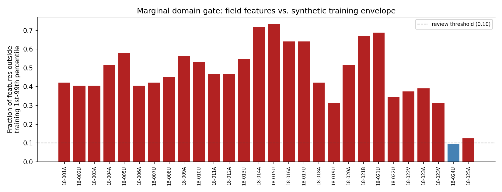
Twenty-seven of the twenty-eight stations exceed the 10% review threshold; only one falls inside it. A synthetic training envelope built from a generic noise model is not automatically wide enough for a real survey.#
Equation (1) is only a marginal, per-feature gate on the synthetic percentile envelope, and it is common for real field data to sit partly outside a generic synthetic prior even when the predictions themselves remain usable. Strongly correlated feature patterns can also remain out of domain even when every value lies inside its individual range. Where available, also apply multivariate distance, latent-space, density, ensemble disagreement, missingness, and geometry checks — this bar chart is a first screen, not the final word.
The package supplies multivariate screens through
flag_out_of_distribution(). Apply them in the
same feature representation used to define the reference set:
>>> from pycsamt.ai.validation import flag_out_of_distribution
>>> training_features = np.load(
...     "model_package/training_features_pre_normalization.npy"
... )
>>> ood = flag_out_of_distribution(
...     X_field, training_features, method="knn", k=5, quantile=0.99
... )
>>> ood.scores.shape, round(ood.fraction_flagged, 3)
((28,), 0.964)
knn uses distance to the \(k\)-th training neighbour and derives its
threshold from leave-one-out training distances. mahalanobis measures
distance in the training covariance geometry and requires more reference rows
than features plus a nonsingular covariance. Neither score is a probability;
feature scaling, reference selection, \(k\), method, and threshold are
part of the approved gate.
Define actions in advance:
accept_for_predictionInput falls inside validated operating conditions.
predict_with_reviewLimited departure exists, prediction is retained for expert evaluation, and the departure is visible in outputs.
rejectInput is incompatible or materially outside the validated domain.
Do not use the visual plausibility of the prediction to override an input gate without documenting a new review decision.
6.3.15.9. 8. Run 1-D prediction#
Raw parameter vectors#
>>> y_pred = inverter.predict(X_field, as_log_rho=True)
>>> y_pred.shape
(28, 9)
The output contains resistivity parameters first and thickness parameters
after them — for this 5-layer checkpoint, that is 5 log10-resistivity values
followed by 4 thickness values, concatenated into one length-9 row. With
as_log_rho=True, resistivity remains log10 ohm metres. Thickness behavior
depends on the fitted inverter’s log_thickness setting (True here).
Do not assume the entire output vector has one unit — the same raw-vector
layout resurfaces for GCNInverter3D in
10. Run graph 3-D prediction below, and slicing it incorrectly there
silently mixes resistivity and thickness together.
With as_log_rho=False, the method converts resistivity to linear ohm metres
and converts thickness to linear metres when log_thickness is enabled.
LayeredModel output#
Prefer pycsamt.ai.inversion.EMInverter1D.predict_models() when downstream
code expects physical layered models:
>>> models = inverter.predict_models(X_field)
>>> sum(1 for m in models if m is None)
0
>>> models[0].resistivity.round(1), models[0].thickness.round(1)
(array([  327.2,   647.8,  5680.7,  2609.5, 1041267.2]), array([ 29.5, 374.2, 256.3, 284.8]))
This method back-transforms resistivity and thickness, clips resistivity to a
positive minimum and thickness to at least one metre, and can return None
when model construction fails. Clipping should be reported; a boundary value
may signal unsupported output rather than a physical estimate. A deep,
resistive basement layer such as station 18-001A’s \(10^{6}\)-scale final
value is physically plausible for crystalline basement, but it is exactly the
kind of boundary-adjacent estimate that response reconstruction (step 15)
should confirm rather than accept on inspection alone.
Single synthetic response#
predict_response(response) is a convenience for a compatible
ForwardResponse. Field Sites should use the public
bridge so station identity and interpolation remain explicit.
6.3.15.10. 9. Run 2-D profile prediction#
Create the field panel with the contract used during training:
>>> from pycsamt.ai.inversion import sites_to_panel_2d
>>> X_profile, frequencies_hz, station_names = sites_to_panel_2d(
...     sites,
...     n_freqs=32,
...     n_components=2,
...     comp_te="xy",
...     comp_tm="yx",
...     freq_min=1.05,
...     freq_max=9500.0,
... )
>>> section = inverter_2d.predict(X_profile, as_log_rho=True)
>>> X_profile.shape, section.shape
((1, 2, 32, 28), (1, 40, 28))
Plot the returned section with one declared transformation and fixed limits; letting each deployment choose its own colour range makes comparisons misleading:
>>> import matplotlib.pyplot as plt
>>> fig, ax = plt.subplots(figsize=(11.0, 5.0))
>>> image = ax.imshow(section[0], aspect="auto", origin="upper",
...                   cmap="turbo", vmin=0.0, vmax=4.0)
>>> _ = ax.set(
...     xlabel="Station index", ylabel="Depth-cell index",
...     title="Predicted 2-D log-resistivity section",
... )
>>> _ = fig.colorbar(image, ax=ax, label="log10 resistivity [ohm m]")
>>> fig.tight_layout()
>>> plt.show()
The input shape is (n_profiles, n_components, n_freqs, n_stations). The
output shape is (n_profiles, n_depth, n_stations). n_components=2 is
deliberate here, not a shortcut: the public 2-D synthetic generator behind a
freshly trained EMInverter2D produces log10
apparent resistivity and phase for one component, not four Re/Im tensor
channels, so a panel and a training target must agree on that count before
fit() is ever called.
No captured section is shown here, unlike the 1-D and 3-D examples elsewhere
on this page: those load a persisted, reviewed checkpoint (step 4), while
inverter_2d above has no such checkpoint step to demonstrate and would
have to be refit from scratch for this example. A U-Net trained on a small
synthetic realization budget for a handful of epochs, with the spatial
regularization weights (lambda_x, lambda_z, lambda_tv –
(3) in AI inversion agents) left at their zero
default, has no architectural or loss-level reason to keep neighbouring
stations coherent, and running it against real field data rather than a
held-out synthetic sample adds a domain-shift gap on top of that. The
result is a section that looks like per-station noise rather than a smooth
or even a plausibly blurry profile – not a plotting bug, and not evidence
that EMInverter2D is unsuitable, but not a result worth publishing
either. Run the code above yourself against your own trained (and ideally
checkpointed) inverter_2d and inspect what you actually get, rather than
trusting a placeholder capture from an unreviewed retrain.
The 2-D inverter applies its learned input and target normalization internally. The field station count must match the inverter’s configured station axis. Station ordering is preserved by the bridge and must already follow reviewed profile chainage.
In the current implementation, each of _x_mean, _x_std, _y_mean,
and _y_std is one scalar computed over the complete training tensor, not a
per-channel or per-frequency array. predict reuses those saved scalars.
Although fitting computes them with nanmean/nanstd, normalization does
not remove missing cells: a nan remains nan and propagates through the
network. A finite-value or validated imputation gate is therefore required
before both fitting and inference.
Use as_log_rho=False for linear ohm metres. Retain the fixed depth grid
from model metadata; the predicted array alone does not contain depth
coordinates.
The fitted 2-D model can be persisted through the BaseEMNet interface inherited by
EMInverter2D:
>>> inverter_2d.save("checkpoints/line2d_unet.npz")
>>> restored_2d = type(inverter_2d).load(
...     "checkpoints/line2d_unet.npz"
... )
>>> restored_2d.n_depth, restored_2d.n_stations, restored_2d.n_freqs
(40, 28, 32)
The checkpoint carries architecture parameters, backend weights, channel
selection, and fitted scalar input/target normalization. It does not turn the
frequency values, station identities, profile chainage, component convention,
depth coordinates, training distribution, or validation decision into an
inference manifest. Preserve those scientific contracts beside the checkpoint
and check them before calling predict.
6.3.15.11. 10. Run graph 3-D prediction#
Graph prediction requires features plus adjacency or coordinates:
>>> from pycsamt.ai.inversion import (
...     sites_to_coords_3d,
...     sites_to_features_1d,
... )
>>> X_nodes, frequencies_hz, station_names = sites_to_features_1d(
...     sites,
...     comp="xy",
...     n_freqs=32,
...     freq_min=1.05,
...     freq_max=9500.0,
... )
>>> coords_m = sites_to_coords_3d(sites, station_spacing=500.0)
>>> graph_prediction = inverter_3d.predict(
...     X_nodes,
...     coords=coords_m,
...     radius=250.0,
...     as_log_rho=True,
... )
>>> graph_prediction.shape
(28, 9)
The network call itself does not run Maxwell physics. The checkpoint must
state whether its training responses came from tiled MT1D columns,
MT3DAdapter, or a solver-neutral corpus produced with
ModEm3DAdapter. All three checkpoints may share the same GCN architecture
and output shape while representing materially different training
distributions. The inference record must therefore preserve the dataset
manifest and forward-backend identity; a generic label such as gcn3d or
physics=mt3d is not enough to establish that ModEM generated the training
responses.
The field feature order, coordinate order, and station-name order must be
identical. sites_to_coords_3d reads each station’s EDI header coordinates
and projects them to local metres; it falls back to an artificial uniform
line only when a station’s coordinates are genuinely absent or all zero — do
not assume a fallback layout is in effect just because the numbers look
large, since the projection here is an absolute equirectangular approximation
rather than one centred on a local origin.
Like the 2-D estimator, the current GCN stores one global scalar mean and standard deviation for all input values and another pair for all target values. This is the implemented contract, even when feature blocks have different physical meanings. Do not replace it at inference with per-feature standardization unless the model is retrained and revalidated with that new contract.
Like the 1-D raw vector in step 8, graph_prediction concatenates
resistivity first and thickness second — (n_stations, 2 * n_layers - 1),
9 columns for these 5-layer models. Split it explicitly before treating any
part of it as a resistivity section:
>>> n_layers = 5
>>> pred_rho = graph_prediction[:, :n_layers]
>>> pred_rho.min().round(2), pred_rho.max().round(2)
(-1.61, 6.29)
pred_rho has shape (station, layer). It is a set of graph-coupled
vertical columns, not yet a rectilinear (z, y, x) resistivity volume. The
layer depths come from each row’s predicted thickness block; if thickness
varies by station, even the vertical cell boundaries are not shared until a
declared resampling is applied. Creating a map volume requires an explicit
operator
where \(\mathbf c_s\) are station coordinates and \(\mathbf h_{s\ell}\) are layer thicknesses. Record the target output grid, interpolation or support radius, extrapolation rule, and cells with no station support. Equation (2) is a display/model-transfer step; it does not add spatial resolution or turn the prediction into a numerical 3-D inversion.
If the fitted inverter stored an approved adjacency matrix, omit new geometry only when field nodes and order are exactly the same. Otherwise pass a reviewed adjacency explicitly:
>>> graph_prediction = inverter_3d.predict(
...     X_nodes,
...     adjacency=approved_adjacency,
...     as_log_rho=True,
... )
Inspect graph degree and disconnected nodes. Changing radius changes the
model context and is not a harmless inference option.
The graph inverter also inherits save()/load(). Its checkpoint includes
network weights, fitted scalar normalization, backend, and the adjacency stored
during fit when one exists:
>>> inverter_3d.save("checkpoints/survey_gcn.npz")
>>> restored_3d = type(inverter_3d).load(
...     "checkpoints/survey_gcn.npz"
... )
>>> restored_3d.n_features, restored_3d.n_layers
(64, 5)
Coordinates, station names, coordinate reference system, radius-based graph construction policy, and the meaning of every feature and output column still belong in the external deployment record. When a stored adjacency is reused, verify its shape and station ordering against the inference survey; a valid matrix attached to the wrong node order is scientifically invalid without raising a shape error.
Elevation deserves the same separation. sites_to_coords_3d returns
horizontal coordinates for graph construction; draping the decoded columns
over station elevation changes their presentation, not the forward physics.
Neither inference nor gridding introduces inactive air cells. A
terrain-physics claim requires a separately constructed, terrain-capable
Maxwell problem and a backend validated for it; the current MT2D, MT3D, and v1
ModEM adapters do not provide that capability.
6.3.15.12. 11. Predict graph uncertainty#
Use Monte Carlo dropout where supported:
>>> mean, standard_deviation = inverter_3d.predict_with_uncertainty(
...     X_nodes,
...     coords=coords_m,
...     radius=250.0,
...     n_mc=40,
... )
>>> std_rho = standard_deviation[:, :n_layers]
>>> float(std_rho.mean().round(3))
0.11
Verify the exact signature in the installed API when passing adjacency versus coordinates. The standard deviation is in output-parameter space — slice it to the resistivity block exactly as in step 10 — and should be reported with the same transformation as the mean. It captures stochastic dropout variation only, one epistemic uncertainty estimate among several, not total inversion or domain uncertainty.
6.3.15.13. 12. Ensemble inference#
pycsamt.ai.inversion.EnsembleInverter can return a mean, spread,
quantiles, intervals, or calibrated posterior draws:
>>> from pycsamt.ai.inversion import EnsembleInverter
>>> ensemble = EnsembleInverter.load("checkpoints/mt1d_ensemble")
>>> mean = ensemble.predict(X_field)
>>> mean, std = ensemble.predict_with_uncertainty(X_field)
>>> quantiles = ensemble.predict_quantiles(X_field, q=(0.05, 0.50, 0.95))
>>> mean.shape, std.shape
((28, 9), (28, 9))
An ensemble has explicit save() and load() support. Its members must
share a compatible input and output contract. The current serialization stores
member checkpoints, estimator count, and seeds; it does not serialize the
attached conformal or posterior calibrators.
After loading, restore calibration through the project’s reviewed
calibration set and call calibrate() again before requesting
intervals:
>>> cal = np.load("checkpoints/mt1d_ensemble_cal_set.npz")
>>> _ = ensemble.calibrate(cal["X_cal"], cal["y_cal"], alpha=0.10)
>>> mean, std = ensemble.predict_with_uncertainty(X_field)
>>> std[0, :5].round(3)
array([0.257, 0.189, 0.05 , 0.081, 0.158])
For a single station, plot interval bounds against layer index without first converting only the mean to linear resistivity:
>>> import matplotlib.pyplot as plt
>>> station_index = 0
>>> layer = np.arange(1, inverter.n_layers + 1)
>>> center = mean[station_index, :inverter.n_layers]
>>> spread = std[station_index, :inverter.n_layers]
>>> lower90 = center - 1.645 * spread
>>> upper90 = center + 1.645 * spread
>>> fig, ax = plt.subplots(figsize=(5.4, 5.0))
>>> _ = ax.errorbar(
...     center, layer, xerr=[center - lower90, upper90 - center],
...     fmt="o-", capsize=3,
... )
>>> ax.invert_yaxis()
>>> _ = ax.set(xlabel="log10 resistivity [ohm m]", ylabel="Layer index")
>>> fig.tight_layout()
>>> plt.show()
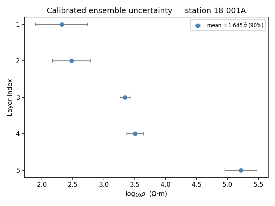
Layer-by-layer calibrated uncertainty for station 18-001A. Interval width grows with depth, consistent with declining sensitivity as period increases — a shallower, better-resolved layer should show a tighter band than the half-space estimate beneath it.#
predict_intervals() uses a
different calibrator — split conformal prediction — built around one
shared multiplier \(\hat q\) applied to every output dimension at once:
Equation (3) takes the worst normalised residual across all 9 output dimensions and gives a valid joint guarantee, but it means one badly scaled dimension inflates every other dimension’s interval too:
>>> center, lower, upper = ensemble.predict_intervals(X_field, alpha=0.10)
>>> lower[0, :5].round(1), upper[0, :5].round(1)
(array([-8233.4, -6040.6, -1608.2, -2606.9, -5070. ]), array([8238. , 6045.6, 1614.9, 2613.9, 5080.4]))
Compare that to the calibrated std-based interval above: the resistivity
parameters are perfectly well behaved (std of a few tenths of a
log10-unit), but because this same target vector also carries linear-metre
thickness values two to three orders of magnitude larger, the single
\(\hat q\) needed to cover the worst thickness dimension dwarfs the
resistivity intervals into physical nonsense. Read this as a warning about
\(\hat q\)’s joint-max design when a target mixes incompatible units, not
as a property of the resistivity estimate itself — the calibrated
predict_with_uncertainty above and predict_posterior below both scale
each output dimension by its own residual spread and stay interpretable.
>>> posterior_draws = ensemble.predict_posterior(
...     X_field, n_samples=500, rng=np.random.default_rng(42),
... )
>>> posterior_draws.shape
(500, 28, 9)
>>> posterior_draws[:, 0, :5].std(axis=0).round(3)
array([0.262, 0.178, 0.049, 0.08 , 0.157])
Conformal coverage assumes calibration and deployment examples are exchangeability-compatible. The convenience method below does not evaluate the conformal interval from equation (3); it measures how often targets fall inside the mean plus or minus the default 1.96 calibrated standard deviations. On this reference calibration set that separate Gaussian-style diagnostic was only 12.3%:
>>> ensemble.coverage(cal["X_cal"], cal["y_cal"])
0.123
That gap is not uniform across output dimensions — the resistivity
parameters cover far better than the thickness parameters, which this
ensemble’s raw inter-member spread represents poorly. A single pooled
coverage number can hide exactly this kind of per-parameter split. Evaluate
conformal coverage directly from lower <= y <= upper when reporting the
conformal method, and distinguish marginal, simultaneous-vector, and
per-parameter coverage. Preserve the calibration dataset ID and empirical
test coverage, broken out by output
dimension where practical, with the inference output. Do not assume a loaded
ensemble remains calibrated merely because the ensemble directory was saved
after calibration.
Reliability and sharpness answer different questions#
For Gaussian predictive summaries, a nominal central interval of level \(c\) is
where \(\Phi^{-1}\) is the standard-normal quantile. On an independent held-out set with validity mask \(M\), empirical coverage is
A reliable predictor follows \(\widehat C(c)\approx c\) over several
levels. Sharpness measures interval concentration–implemented by
predictive_sharpness() as mean predictive
standard deviation–and is useful only after reliability is acceptable. An
arbitrarily tiny standard deviation is very sharp and very wrong whenever it
fails to cover held-out truth.
The executed diagnostic below uses
reliability_curve() on 720 synthetic held-out
layer parameters. Both candidates have the same predictive mean. One reports
the data-generating uncertainty scale; the other reports only 45% of it. The
exact figure code is exposed so the arrays can be replaced with calibration or
test outputs from a real model package.
View calibration-diagnostic source codeClick to inspect and copy the complete code
 1def make_inference_calibration_diagnostic() -> None:
 2    """Compare calibrated and overconfident predictive distributions."""
 3    from scipy.stats import norm
 4
 5    from pycsamt.ai.validation import reliability_curve
 6
 7    rng = np.random.default_rng(2026)
 8    n_station, n_layer = 120, 6
 9    depth = np.arange(1, n_layer + 1)
10    mean = 1.55 + 0.27 * depth[None, :] + rng.normal(
11        0.0, 0.08, size=(n_station, 1)
12    )
13    true_sigma = 0.07 + 0.035 * depth[None, :]
14    true_sigma = np.broadcast_to(true_sigma, mean.shape)
15    truth = mean + rng.normal(size=mean.shape) * true_sigma
16    calibrated_std = true_sigma.copy()
17    overconfident_std = 0.45 * true_sigma
18    levels = np.linspace(0.10, 0.99, 18)
19    calibrated = reliability_curve(
20        truth, mean, calibrated_std, levels=levels, kind="l1"
21    )
22    overconfident = reliability_curve(
23        truth, mean, overconfident_std, levels=levels, kind="l1"
24    )
25
26    fig, axes = plt.subplots(1, 3, figsize=(13.2, 4.3))
27    axes[0].plot(levels, levels, "k--", label="ideal")
28    axes[0].plot(
29        calibrated.levels, calibrated.coverage, "o-", label="calibrated scale"
30    )
31    axes[0].plot(
32        overconfident.levels,
33        overconfident.coverage,
34        "s-",
35        label="45% uncertainty scale",
36    )
37    axes[0].set(
38        xlabel="Nominal coverage",
39        ylabel="Empirical coverage",
40        title="Reliability is measured against truth",
41        xlim=(0, 1),
42        ylim=(0, 1),
43    )
44    axes[0].grid(alpha=0.25)
45    axes[0].legend(fontsize=8)
46
47    station = 7
48    z90 = norm.ppf(0.95)
49    axes[1].plot(mean[station], depth, "ko-", label="predictive mean")
50    axes[1].fill_betweenx(
51        depth,
52        mean[station] - z90 * calibrated_std[station],
53        mean[station] + z90 * calibrated_std[station],
54        alpha=0.25,
55        label="calibrated 90% interval",
56    )
57    axes[1].scatter(truth[station], depth, c="#dc2626", zorder=3, label="truth")
58    axes[1].invert_yaxis()
59    axes[1].set(
60        xlabel=r"$\log_{10}\rho$ [$\Omega\cdot$m]",
61        ylabel="Layer index",
62        title="One synthetic held-out station",
63    )
64    axes[1].grid(alpha=0.25)
65    axes[1].legend(fontsize=8)
66
67    labels = ["calibrated\nscale", "overconfident\nscale"]
68    calibration_error = [
69        calibrated.calibration.value,
70        overconfident.calibration.value,
71    ]
72    sharpness = [calibrated.sharpness, overconfident.sharpness]
73    x = np.arange(2)
74    axes[2].bar(x - 0.18, calibration_error, 0.36, label="mean |coverage error|")
75    axes[2].bar(x + 0.18, sharpness, 0.36, label="sharpness (mean std)")
76    axes[2].set_xticks(x, labels)
77    axes[2].set(
78        ylabel="Diagnostic value",
79        title="Sharper is not better when miscalibrated",
80    )
81    axes[2].grid(alpha=0.25, axis="y")
82    axes[2].legend(fontsize=8)
83    fig.suptitle(
84        "Inference uncertainty audit on 720 held-out layer parameters",
85        fontsize=13,
86    )
87    fig.tight_layout()
88    _save(fig, "inference_calibration_diagnostic.png")
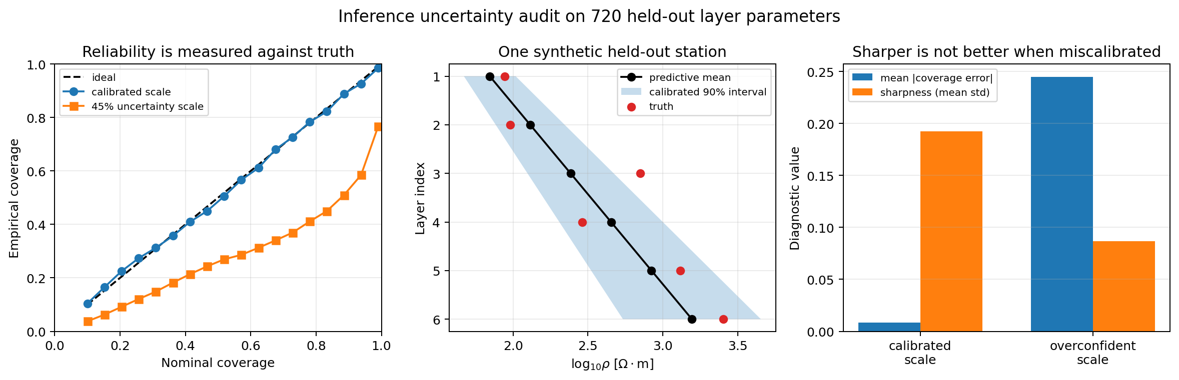
Executed comparison of a calibrated uncertainty scale and an overconfident scale for identical predictive means.#
The calibrated curve stays close to the diagonal, with mean absolute coverage error 0.009 and mean standard deviation 0.193 log10 ohm metres. Shrinking the standard deviations makes the result look sharper (0.087) but raises coverage error to 0.245; even the nominal 99% intervals cover only 76.7% of held-out parameters. The middle panel also shows why one station is not a calibration test: a few truths can fall inside or outside by chance. Reliability is an ensemble property measured on untouched examples, then stratified by layer, parameter type, domain status, and decision-relevant subgroup.
6.3.15.14. 13. PINN and hybrid inference#
PINN and hybrid classes do not follow the same stateless predict(X) pattern
as supervised surrogates: both are constructed directly from sites and
require an explicit fit() call before predict() returns anything.
pycsamt.ai.inversion.PINNInverter1D.predict then returns fitted
layered models after observation-specific optimization, and
pycsamt.ai.inversion.HybridInverter1D.predict returns the refined
models associated with its configured observations:
>>> from pycsamt.ai.inversion import PINNInverter1D
>>> pinn = PINNInverter1D(
...     "data/AMT/WILLY_data/L18PLT", solver="mt1d", n_layers=10,
...     depth_max=2000.0, smoothness_weight=0.01, lr=1e-2, comp="xy",
... )
>>> _ = pinn.fit(epochs=400, verbose=False)
>>> pinn_models = pinn.predict()
>>> len(pinn_models), sum(1 for m in pinn_models if m is None)
(28, 0)
>>> pinn_models[0].resistivity.round(0)
array([ 100.,  957.,  623.,  821.,  622.,  821.,  622.,  821.,  622., 821.])
Ten layers were requested, but from the third layer down the values settle into an alternating ~623/~821 pattern rather than resolving independently — a visible symptom of non-uniqueness: past a certain depth the smoothness-regularised physics loss stops discriminating between layer configurations that produce nearly the same surface response, and the optimizer parks on one arbitrary member of that family. Report the depth beyond which layers stop varying independently rather than presenting all ten as equally resolved.
>>> from pycsamt.ai.inversion import HybridInverter1D
>>> hybrid = HybridInverter1D(
...     "data/AMT/WILLY_data/L18PLT",
...     ai_inverter="checkpoints/mt1d_resnet_5layer.npz",
...     solver="mt1d", max_iter=150, smoothness_weight=0.005,
...     lr=5e-3, comp="xy", n_freqs=32,
... )
>>> _ = hybrid.fit(verbose=False)
>>> hybrid_models = hybrid.predict()
>>> hybrid_models[0].resistivity.round(1)
array([1.348e+02, 5.770e+02, 3.793e+03, 2.258e+03, 1.117e+05])
The hybrid result stays close to the plain checkpoint’s own prediction for
this station (compare step 8’s [327, 648, 5681, 2610, 1.04e6]) while
refining it against the physics residual — starting from a trained AI
estimate rather than an arbitrary initial model is exactly the point of the
two-stage design, and a hybrid result that looks nothing like its AI starting
point is worth investigating before it is trusted.
Treat both as inversion runs rather than pure checkpoint deployment:
preserve observations and optimizer configuration;
verify convergence and loss components;
record regularization and initialization;
inspect fitted responses and per-station residuals;
do not reuse a result for different observations without rerunning the documented workflow.
See Physics-informed 2-D inversion for the complete profile workflow.
6.3.15.15. 14. Decode outputs safely#
Every exported array needs a schema. Record:
array shape and axis names;
station order;
depth/layer coordinates;
parameter block boundaries;
log10 versus linear values;
resistivity and thickness units;
masked, rejected, or clipped predictions;
model/checkpoint identifier;
preprocessing and inference version.
For the five-layer checkpoint, decoding raw row \(\mathbf y\) is
Equation (6) is model metadata in mathematical form; guessing the second branch from numerical magnitude can silently turn metres into powers of ten.
Validate decoded properties:
>>> for name, model in zip(station_names, models):
...     if model is None:
...         continue
...     if not np.all(np.isfinite(model.resistivity)):
...         raise ValueError(f"{name}: non-finite resistivity")
...     if not np.all(model.resistivity > 0):
...         raise ValueError(f"{name}: non-positive resistivity")
...     if not np.all(model.thickness > 0):
...         raise ValueError(f"{name}: non-positive thickness")
No error raised for these 28 stations — but positive and finite values are necessary, not sufficient. Also compare with training bounds and flag predictions near limits, such as station 18-001A’s basement resistivity above.
6.3.15.16. 15. Reconstruct forward responses#
A predicted model should be passed through the relevant forward operator and compared with field observations. For layered MT:
>>> from pycsamt.forward import MT1DForward
>>> reconstructed = []
>>> for model in models:
...     if model is None:
...         reconstructed.append(None)
...         continue
...     reconstructed.append(MT1DForward(freqs=frequencies_hz).run(model))
Calculate residuals in a clearly defined space. A robust report states:
apparent resistivity, phase, complex impedance, or decay values used;
linear or log residual transformation;
observational errors and weights;
interpolation grid;
components included;
missing-data mask;
global and station/frequency summaries.
When standard deviations \(\sigma_i\) are available, one comparable summary is the normalized RMS
Report equation (7) separately by component and useful frequency band as well as globally. A single average can still hide where a structured residual occurs.
Do not accept a model solely because it resembles expected geology. Conversely, response agreement alone cannot establish uniqueness — as the PINN layers in step 13 make concrete.
For a graph checkpoint, choose the reconstruction operator according to the
claim being tested. Station-wise MT1DForward responses test whether each
decoded column is locally compatible with the observations, but they do not
test the lateral coupling represented during genuine 3-D Maxwell training.
To audit that claim, first apply the documented graph-to-grid mapping from
equation (2), transfer the result onto a
solver mesh, and solve the shared 3-D conductivity model with
MT3DAdapter for a research-scale check or ModEm3DAdapter for the
production backend. Compare the requested tensor components on the observed
frequency and station axes, preserving observational errors and masks.
That 3-D reconstruction is currently an explicit workflow, not a method
inside GCNInverter3D.predict. Its result must retain the graph prediction,
mapping configuration, Maxwell problem hash, backend/version, diagnostics,
and residual table. ModEM’s v1 diagnostic residual of zero is a documented
placeholder because its predicted-data file exposes no algebraic residual;
use response benchmarks and observed-data residuals as the evidence instead.
6.3.15.17. 16. Apply acceptance rules#
Combine gates rather than relying on one RMS:
- Input compatibility
Exact feature contract, finite values, frequency support, geometry, and accepted missingness.
- Domain support
Training-envelope, multivariate, latent, or ensemble diagnostics.
- Output validity
Finite physical parameters, supported bounds, no unexplained clipping, and correct shape.
- Response fit
Error-aware reconstructed response with no structured residual pattern.
- Uncertainty
Calibrated interval or model spread suitable for the decision.
- Scientific consistency
Dimensionality, classical baseline, boreholes, geology, and neighboring observations.
Assign accepted, needs_review, or rejected per station/profile and
preserve the reason. Do not remove rejected stations from exports without a
rejection table.
6.3.15.18. 17. Batch and resource behavior#
For 1-D models, batch size affects memory and throughput but should not change station semantics. Confirm numerical consistency between a small batch and the production batch.
For 2-D and graph models, one batch item contains a complete profile or survey. Padding multiple geometries to one size requires a trained mask policy.
Run inference in evaluation mode. The provided supervised prediction methods handle backend evaluation internally. MC dropout intentionally reintroduces stochastic behavior for uncertainty; use a documented sample count and seed where the API permits.
Record device, backend, precision, batch size, elapsed time, and memory-related fallbacks. Numerical differences across devices should be evaluated against an approved tolerance.
6.3.15.19. 18. Export an inference record#
A reproducible inference directory can contain:
inference/L18_mt1d_resnet_v001/
├── manifest.yml
├── checkpoint_reference.yml
├── input/
│   ├── station_inventory.csv
│   ├── field_features.npz
│   └── domain_diagnostics.csv
├── predictions/
│   ├── parameter_vectors.npz
│   ├── layered_models.csv
│   └── status_by_station.csv
├── responses/
│   └── reconstructed_residuals.csv
├── uncertainty/
│   └── prediction_intervals.npz
├── figures/
└── review/
    └── inference_review.md
The manifest should record checkpoint checksum, feature contract, input survey and QC IDs, preprocessing version, domain thresholds, software/backend, device, random settings, output schema, accepted/rejected stations, reviewer, status, and date.
6.3.15.20. Complete 1-D inference example#
>>> from pathlib import Path
>>> import json
>>> import numpy as np
>>> from pycsamt.ai.inversion import EMInverter1D, sites_to_features_1d
>>> from pycsamt.emtools._core import ensure_sites
>>> from pycsamt.forward import MT1DForward
>>> root = Path("inference/L18_mt1d_resnet_v001")
>>> root.mkdir(parents=True, exist_ok=True)
>>> inverter = EMInverter1D.load("checkpoints/mt1d_resnet_5layer.npz")
>>> sites = ensure_sites("data/AMT/WILLY_data/L18PLT", recursive=True, verbose=0)
>>> X, freqs, names = sites_to_features_1d(
...     sites, comp="xy", n_freqs=32, freq_min=1.05, freq_max=9500.0,
... )
>>> # Replace this gate with the approved model-package policy.
>>> finite_fraction = np.mean(np.isfinite(X), axis=1)
>>> accepted = finite_fraction == 1.0
>>> int(accepted.sum())
28
>>> models = [None] * len(names)
>>> if accepted.any():
...     accepted_models = inverter.predict_models(X[accepted])
...     for index, model in zip(np.flatnonzero(accepted), accepted_models):
...         models[index] = model
>>> responses = []
>>> forward = MT1DForward(freqs=freqs)
>>> for model in models:
...     responses.append(None if model is None else forward.run(model))
>>> rho = np.full((len(names), inverter.n_layers), np.nan)
>>> thickness = np.full((len(names), inverter.n_layers - 1), np.nan)
>>> for index, model in enumerate(models):
...     if model is not None:
...         rho[index] = model.resistivity
...         thickness[index] = model.thickness
>>> np.savez_compressed(
...     root / "predictions.npz",
...     station_names=np.asarray(names),
...     frequencies_hz=freqs,
...     resistivity_ohm_m=rho,
...     thickness_m=thickness,
...     accepted=accepted,
... )
>>> manifest = {
...     "checkpoint": "mt1d_resnet_5layer.npz",
...     "component": "xy",
...     "n_freqs": 32,
...     "freq_min_hz": 1.05,
...     "freq_max_hz": 9500.0,
...     "feature_layout": "log10_rho_then_phase_deg",
...     "accepted_stations": int(accepted.sum()),
...     "rejected_stations": int((~accepted).sum()),
... }
>>> _ = (root / "manifest.json").write_text(
...     json.dumps(manifest, indent=2), encoding="utf-8",
... )
Because the field query grid was matched to the checkpoint’s own training band (step 5), every station clears the strict all-finite gate here — a direct contrast with the 56.25%-nonfinite result a mismatched grid would have produced, and with the 27-of-28 review flags the percentile gate in step 7 raises on the very same stations. A production model may use a different approved policy for either gate, but it must not improvise one during deployment.
6.3.15.21. Review checklist#
Check |
Required evidence |
|---|---|
Model is approved |
Identifier, checksum, model card, validation, calibration, and status. |
Contract matches |
Method, features, grid, normalization, output schema, and geometry. |
Inputs are traceable |
Survey, QC, processing, station order, coordinates, and exclusions. |
Missingness follows policy |
Masks/imputation identical to validation and visible in results. |
Domain gate runs first |
Thresholds, diagnostics, accepted/review/rejected status, and reasons. |
Prediction is immutable |
Evaluation mode, no fitting, no normalization update, and recorded backend/device. |
Outputs decode correctly |
Log/linear conversions, units, layers, depth, station axes, and clipping. |
Responses are reconstructed |
Forward operator, components, errors, residual definition, and patterns. |
Uncertainty is conditional |
Method, calibration set, coverage, domain-shift limitation, and sample count. |
Release is auditable |
Manifest, arrays, status table, checkpoint reference, reviewer, and date. |
6.3.15.22. Common mistakes#
Avoid these errors:
loading an untrusted checkpoint;
checking only feature count rather than feature meaning;
rebuilding normalization from field data;
silently filling NaNs with convenient values;
predicting before out-of-domain screening;
treating all output columns as log10 values;
losing station order when exporting predictions;
changing profile station count or graph radius at deployment;
calling graph-context output a full numerical 3-D inversion;
calling
(station, layer)predictions a rectilinear volume without a documented output-grid mapping and unsupported-cell mask;reporting an MT1D column reconstruction as validation of coupled MT3D response physics, or calling an inference ModEM-generated when only the network ran;
treating an elevation-draped prediction as terrain-aware forward physics;
treating MC dropout or ensemble spread as total uncertainty;
reading a shared-multiplier conformal interval as if it were scaled per-parameter, especially when the target mixes resistivity and thickness;
claiming conformal field coverage from synthetic calibration alone;
accepting geological-looking models without response reconstruction;
exporting predictions without rejected-input records;
loading a 2-D or 3-D checkpoint without restoring its external frequency, station, coordinate, graph, depth, and feature contracts.
6.3.15.23. Next steps#
Continue with:
AI inversion validation for response, baseline, field, and acceptance testing;
AI inversion uncertainty for calibration, ensembles, and distribution shift;
AI inversion reporting for model cards and controlled prediction packages;
AI inversion agents for standard EDI-to-prediction orchestration;
Physics-informed 2-D inversion for observation-specific physics-informed inference.