
6.3.13. AI model selection#
Model selection chooses the scientific representation, learning strategy, and architecture used for AI inversion. It is not simply a search for the network with the lowest validation loss. The selected model must match survey physics, geometry, data volume, target parameterization, deployment constraints, and the evidence required for field acceptance.
pyCSAMT supports supervised 1-D, profile 2-D, graph-context 3-D, joint, ensemble, physics-informed, and hybrid workflows. Each answers a different question and encodes different model prior assumptions. The selection task is therefore a constrained decision:
In equation (1), \(c\) is a candidate workflow and architecture, \(S(c)\) is the predeclared selection score, and \(\mathcal{C}_{\mathrm{valid}}\) contains only candidates that satisfy the survey physics, data contract, validation, deployment, and reproducibility constraints. A model with the smallest synthetic loss is not selectable if it cannot be restored, violates the intended operating envelope, or fails response diagnostics.
Prefer the simplest defensible model
Added architectural complexity is justified only when it improves a predeclared scientific or operational criterion on independent data. A more elaborate network can hide stronger assumptions, increase leakage risk, and make deployment less reproducible without adding recoverable information.
6.3.13.1. Selection workflow#
define the decision, output, and acceptance metrics;
determine defensible physical dimensionality from the survey;
freeze the feature contract and target contract;
establish non-AI and simple AI baseline model comparisons;
identify candidate model families rather than arbitrary hyperparameters;
define leakage-resistant training, validation, calibration, and test roles;
train candidates under comparable budgets;
compare model-space metric, response-space metric, calibration, and field metrics;
test robustness, domain gap, compute, and persistence;
select once using the declared rule and confirm on an untouched test set;
document rejected candidates and the reason for the final choice.
6.3.13.2. 1. Define the selection objective#
Different objectives can select different models. Examples include:
minimize median log-resistivity error on unseen synthetic geology;
recover conductor-top depth within an operational tolerance;
minimize error-weighted field response residuals;
maintain calibrated 90% intervals with useful sharpness;
rank drilling targets consistently across accepted scenarios;
run within memory and latency limits on the deployment machine;
remain stable under missing frequency bands or station dropout.
Declare a primary metric, secondary constraints, and unacceptable failure modes before comparing candidates. Do not select using whichever metric looks best after training. A compact decision score can be useful when it is declared before results are inspected:
In equation (2), the weights \(\alpha\), \(\beta\), and \(\gamma\) do not make the decision objective; the scientific decision makes the weights. For example, a screening tool may tolerate larger model-space error if it is fast and well-calibrated, while a drill-target interpretation may give much more weight to conductor-top depth, response reconstruction, and failure visibility.
6.3.13.3. 2. Decide dimension before architecture#
Dimension is a geophysical assumption, not a neural-network preference. A candidate’s output shape should follow the survey evidence. A useful mental model is
The alternatives in equation (3) control what the model can represent and what it is allowed to ignore. A 1-D model is transparent but cannot represent lateral boundaries. A 2-D profile can represent lateral structure but assumes the line and strike convention are meaningful. A graph-context 3-D model can borrow information from nearby stations, but its graph is a spatial prior and may not mean the training examples used full 3-D electromagnetic physics.
Choose 1-D when#
local geology is approximately layered;
station-by-station screening is the goal;
survey spacing is too sparse for stable lateral learning;
no reviewed profile or areal geometry is available;
a transparent baseline is needed.
Use pycsamt.ai.inversion.EMInverter1D, a 1-D PINN, or a 1-D hybrid.
Document why the 1-D assumption is adequate. If the goal is only screening,
state that; if the result will guide interpretation, pair it with response
residuals and dimensionality diagnostics.
Choose profile 2-D when#
stations form a meaningful ordered line;
tensor, strike, and dimensionality evidence support a 2-D approximation;
lateral continuity is central to the decision;
training examples represent profile geometry and missingness;
a fixed station and depth representation is acceptable.
Use pycsamt.ai.inversion.EMInverter2D,
pycsamt.ai.inversion.PINNInverter2D, or
pycsamt.ai.inversion.HybridInverter2D.
Profile 2-D selection should be tied to the line geometry. Record the station ordering, spacing, strike convention, and how off-line stations are handled. If profiles have variable station counts, choose one validated policy before training: crop, pad, resample, train separate models, or use a graph workflow.
Choose graph-context 3-D when#
stations form several lines or an areal layout;
projected coordinates and station order are reliable;
neighborhood relationships carry useful information;
training surveys represent graph layout and correlation scales;
node-wise layered outputs are suitable.
Use pycsamt.ai.inversion.GCNInverter3D,
pycsamt.ai.inversion.PINNInverter3D, or
pycsamt.ai.inversion.HybridInverter3D.
The GCN shares information among station nodes. It does not automatically mean
that supervised examples were generated with a full numerical 3-D EM solver.
Do not select it merely to label the product “3-D.” Inv3DAgent(physics="mt1d")
(the default) trains on tiled 1-D columns; Inv3DAgent(physics="mt3d")
(3-D Maxwell training-data generation) trains on Genuine 3-D Maxwell training volumes
instead, at substantially higher cost per profile and still only as a
research-stage slice, not a gated production path – see Architecture roadmap’s M8
entry before treating either mode’s output as more validated than it is.
The graph itself is worth inspecting before any physics mode is chosen.
sites_to_coords_3d() and
build_adjacency() are exactly what Inv3DAgent
calls internally, so the adjacency a real run trains on can be built and
read directly:
>>> from pycsamt.emtools._core import ensure_sites
>>> from pycsamt.ai.inversion import sites_to_coords_3d
>>> from pycsamt.ai.nets import build_adjacency

>>> sites = ensure_sites(
...     "data/AMT/WILLY_data/L18PLT", recursive=True, verbose=0
... )
>>> coords = sites_to_coords_3d(sites, recursive=False, verbose=0)
>>> coords.shape
(28, 2)

>>> radius = 250.0
>>> adjacency = build_adjacency(
...     coords, radius, self_loops=False, normalise=False
... )
>>> degree = adjacency.sum(axis=1).astype(int)
>>> int(adjacency.sum() // 2)
65
>>> int((degree == 0).sum())
0
>>> int(degree.min()), int(degree.max())
(2, 7)
At WILLY L18’s own 250 m radius – the same value the executed
physics="mt3d" example in AI inversion agents uses – every station keeps
at least two neighbours, so no node trains in isolation. L18 is a single
profile line rather than an areal layout, which is exactly why its
degree stays modest (2-7) instead of spanning the wide range an areal
survey produces at a fixed radius; the previous diagnostic’s synthetic
points illustrate that areal case deliberately, since a real single-line
survey cannot exercise it. Combining this adjacency with each station’s
own real median measured apparent resistivity, rather than a station
index, shows what the network actually receives as spatial context:
View real WILLY graph-context source codeClick to inspect and copy the complete code
 1def make_gcn_3d_context() -> None:
 2    """The real spatial graph GCNInverter3D/Inv3DAgent build from the real
 3    WILLY L18 station geometry, at the same adjacency radius used by the
 4    executed physics="mt3d" example, coloured by each station's own real
 5    measured apparent resistivity -- not a fabricated synthetic layout.
 6    """
 7    sites = ensure_sites(
 8        PROJECT_ROOT / "data" / "AMT" / "WILLY_data" / "L18PLT",
 9        recursive=True,
10        verbose=0,
11    )
12    coords = sites_to_coords_3d(sites, recursive=False, verbose=0)
13    dense_features, measured_frequency, _ = sites_to_features_1d(
14        sites, comp="xy", n_freqs=64,
15    )
16    # Each station's own median log10 apparent resistivity across the
17    # measured band -- real field data, robust to the ragged per-station
18    # frequency coverage sites_to_features_1d leaves as NaN at the edges.
19    station_log_rho = np.nanmedian(
20        dense_features[:, : measured_frequency.size], axis=1
21    )
22
23    radius = 250.0  # matches Inv3DAgent(physics="mt3d")'s own WILLY example
24    adjacency_raw = build_adjacency(
25        coords, radius, self_loops=False, normalise=False
26    )
27    adjacency_norm = build_adjacency(coords, radius)
28    degree = adjacency_raw.sum(axis=1).astype(int)
29    x, y = coords[:, 0], coords[:, 1]
30    n_stations = coords.shape[0]
31
32    fig = plt.figure(figsize=(10.2, 4.6))
33    ax = fig.add_subplot(111, projection="3d")
34    for i in range(n_stations):
35        for j in range(i + 1, n_stations):
36            if adjacency_raw[i, j] > 0:
37                ax.plot(
38                    [x[i], x[j]],
39                    [y[i], y[j]],
40                    [station_log_rho[i], station_log_rho[j]],
41                    color="#94a3b8",
42                    alpha=0.4,
43                    lw=0.6 + 2.6 * adjacency_norm[i, j],
44                )
45
46    sc = ax.scatter(
47        x,
48        y,
49        station_log_rho,
50        c=station_log_rho,
51        cmap="viridis_r",
52        s=60,
53        edgecolor="#111827",
54        linewidth=0.35,
55        depthshade=False,
56    )
57    ax.set_xlabel("Easting offset (m)")
58    ax.set_ylabel("Northing offset (m)")
59    ax.set_zlabel(r"median $\log_{10}\rho_a$ (measured)")
60    ax.set_title(
61        f"Real GCN spatial graph: WILLY L18, r={radius:.0f} m "
62        f"({int(adjacency_raw.sum() // 2)} edges, "
63        f"{int(np.sum(degree == 0))} isolated)",
64        pad=12,
65    )
66    ax.view_init(elev=16, azim=-70)
67    cb = fig.colorbar(sc, ax=ax, shrink=0.74, pad=0.08)
68    cb.set_label(r"median $\log_{10}\rho_a$ [$\Omega\cdot$m]")
69    fig.tight_layout()
70    _save(fig, "gcn_3d_context.png")
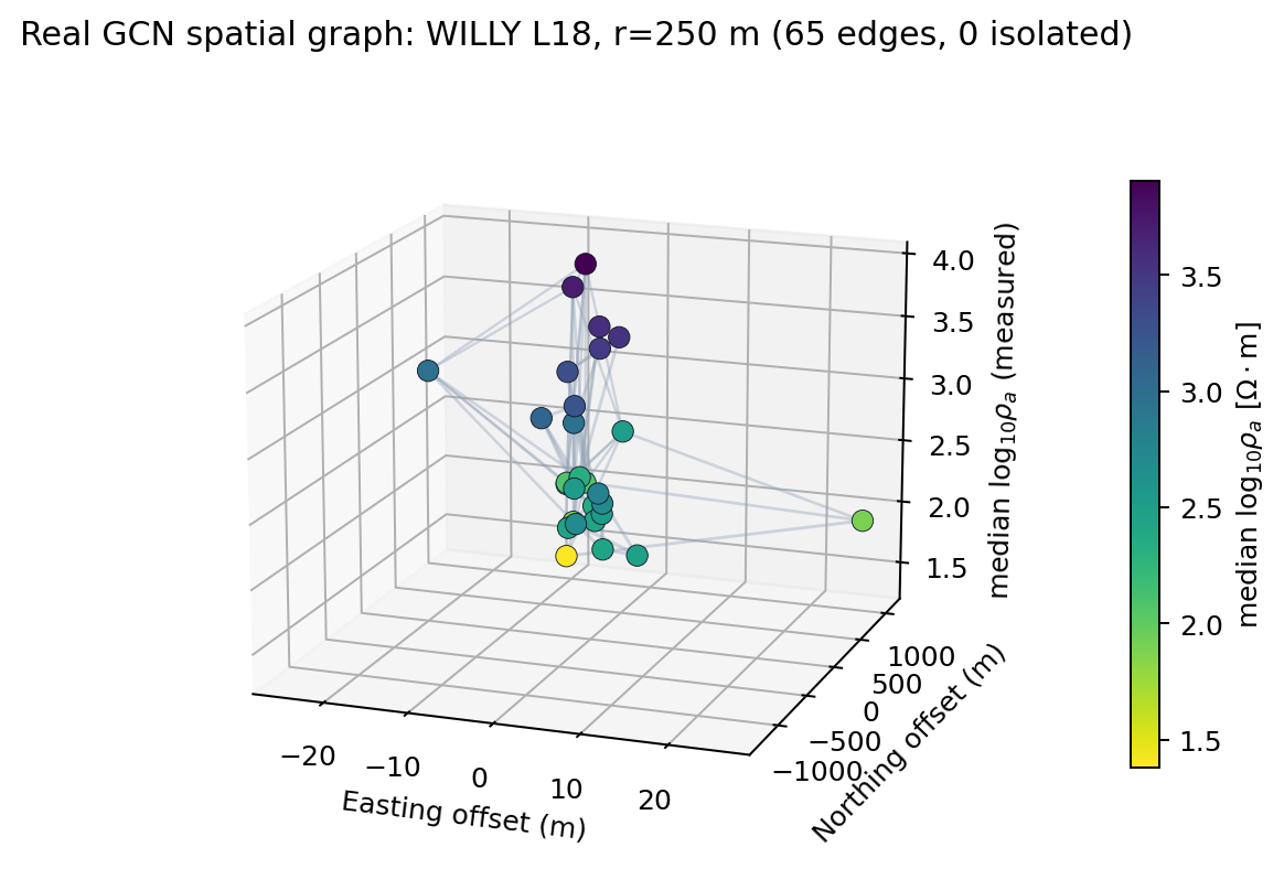
The real spatial graph Inv3DAgent(physics="mt3d") builds from WILLY
L18, not a synthetic layout. Height and colour are each station’s own
median measured \(\log_{10}\rho_a\), not a fabricated feature.#
Edge thickness is the degree-normalised adjacency weight
build_adjacency() itself computes (formalised later
in this page as equation (10)), so a station
with many close neighbours contributes each individual edge more weakly
than one with few. The two
most resistive stations near the profile’s northern end sit close
together and well connected; the lower-resistivity cluster toward the
southern end is denser but locally more uniform. A GCN reading this graph
propagates information along exactly these real edges, not along whichever
lines happened to look tidy in an illustration – which is also why a
degree table like this one belongs in a real run’s own report, not only in
documentation.
When dimension is uncertain, compare conservative alternatives. A common selection record includes a 1-D baseline, a 2-D or graph candidate, and a note explaining whether the higher-dimensional candidate improved a declared criterion enough to justify its stronger assumptions. If the improvement is only cosmetic in section images and not visible in response fit, field evidence, or decision stability, keep the simpler model.
What WILLY L18 permits#
The dimension decision can be exercised on the bundled line before choosing a
network. pycsamt.emtools.dimensionality.classify_dimensionality() uses
phase-tensor skew and ellipticity to classify each usable station-frequency
sample. The labels are a diagnostic under explicit thresholds, not geological
truth, but they reveal whether a layered or strike-invariant assumption is
consistent with the measured tensor.
Writing the complex impedance as \(\mathbf Z=\mathbf X+i\mathbf Y\), the phase tensor and the two plotted invariants are
where \(s_1\ge s_2\) are singular values of \(\boldsymbol\Phi\). The implementation expresses \(\beta\) in degrees and applies the rule
Equations (4) and (5) make the assumptions behind the labels auditable. Changing the thresholds changes the counts and must be justified rather than tuned until a preferred dimension appears.
>>> from pycsamt.emtools._core import ensure_sites
>>> from pycsamt.emtools.dimensionality import classify_dimensionality

>>> sites = ensure_sites(
...     "data/AMT/WILLY_data/L18PLT", recursive=True, verbose=0
... )
>>> dimensionality = classify_dimensionality(sites)
>>> counts = dimensionality["dim"].value_counts().sort_index()
>>> print("station-frequency samples:", len(dimensionality))
station-frequency samples: 1484
>>> print({"1-D": int(counts.get(0, 0)),
...        "2-D": int(counts.get(1, 0)),
...        "3-D": int(counts.get(2, 0))})
{'1-D': 58, '2-D': 155, '3-D': 1271}
>>> print("3-D fraction:", round(float((dimensionality["dim"] == 2).mean()), 3))
3-D fraction: 0.856
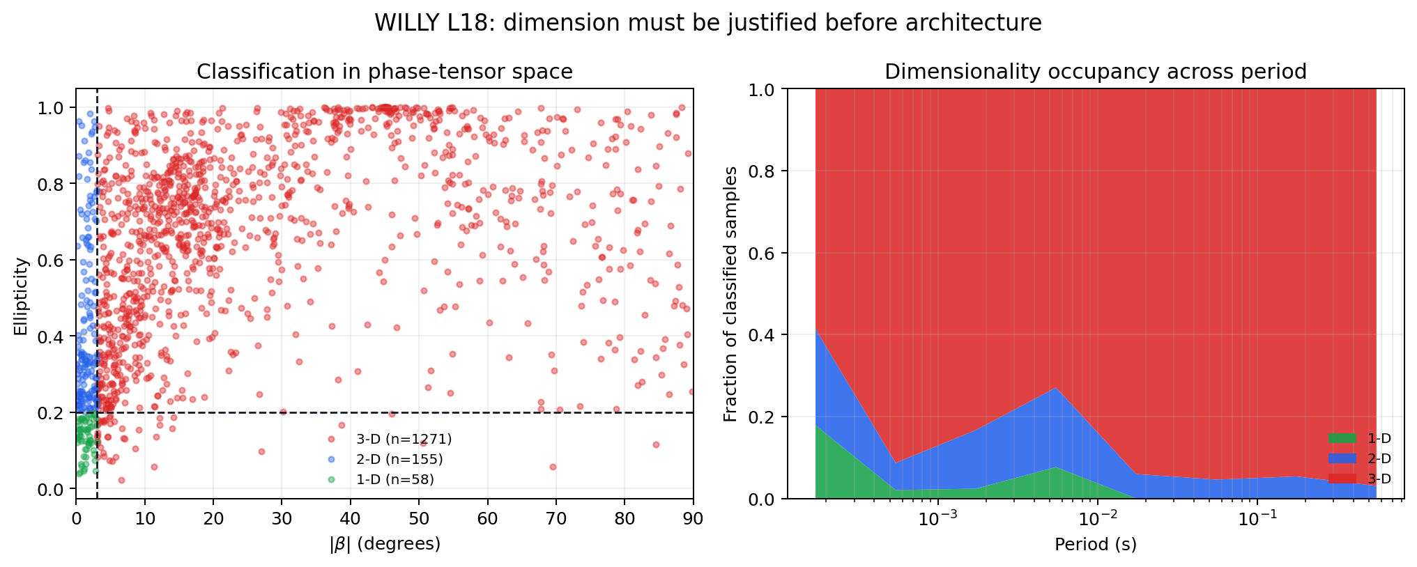
Most samples lie beyond the default 3-degree skew boundary and classify as 3-D. The period-binned panel shows that this is not confined to one narrow band. These labels should be reviewed with strike stability, errors, distortion, source assumptions, and neighboring lines before a physical dimension is accepted.#
The plotting code is intentionally part of the example so the thresholds, period binning, and class counts can be inspected and adapted:
View WILLY dimensionality source codeClick to inspect and copy the complete code
 1def make_model_selection_willy_dimension() -> None:
 2    line = PROJECT_ROOT / "data" / "AMT" / "WILLY_data" / "L18PLT"
 3    sites = ensure_sites(line, recursive=True, verbose=0)
 4    table = classify_dimensionality(sites)
 5    colors = {0: "#16a34a", 1: "#2563eb", 2: "#dc2626"}
 6    names = {0: "1-D", 1: "2-D", 2: "3-D"}
 7
 8    fig, axes = plt.subplots(1, 2, figsize=(11.4, 4.6))
 9    ax_feature, ax_period = axes
10    for label in (2, 1, 0):
11        selected = table["dim"].to_numpy() == label
12        ax_feature.scatter(
13            table.loc[selected, "beta_abs"],
14            table.loc[selected, "ellipt_abs"],
15            s=10,
16            alpha=0.42,
17            color=colors[label],
18            label=f"{names[label]} (n={int(selected.sum())})",
19        )
20    ax_feature.axvline(3.0, color="#111827", ls="--", lw=1.1)
21    ax_feature.axhline(0.2, color="#111827", ls="--", lw=1.1)
22    ax_feature.set(xlabel=r"$|\beta|$ (degrees)", ylabel="Ellipticity")
23    ax_feature.set_xlim(0, 90)
24    ax_feature.set_title("Classification in phase-tensor space")
25    ax_feature.grid(alpha=0.2)
26    ax_feature.legend(frameon=False, fontsize=8)
27
28    period = table["period"].to_numpy(dtype=float)
29    edges = np.logspace(
30        np.log10(np.nanmin(period)), np.log10(np.nanmax(period)), 9
31    )
32    centres = np.sqrt(edges[:-1] * edges[1:])
33    fractions = np.zeros((3, centres.size))
34    for index in range(centres.size):
35        in_bin = (period >= edges[index]) & (period <= edges[index + 1])
36        if np.any(in_bin):
37            labels = table.loc[in_bin, "dim"].to_numpy(dtype=int)
38            fractions[:, index] = [
39                (labels == value).mean() for value in (0, 1, 2)
40            ]
41    ax_period.stackplot(
42        centres,
43        fractions,
44        colors=[colors[0], colors[1], colors[2]],
45        labels=[names[0], names[1], names[2]],
46        alpha=0.88,
47    )
48    ax_period.set_xscale("log")
49    ax_period.set_ylim(0, 1)
50    ax_period.set(xlabel="Period (s)", ylabel="Fraction of classified samples")
51    ax_period.set_title("Dimensionality occupancy across period")
52    ax_period.grid(alpha=0.2, which="both")
53    ax_period.legend(frameon=False, fontsize=8, loc="lower right")
54    fig.suptitle(
55        "WILLY L18: dimension must be justified before architecture",
56        fontsize=13,
57    )
58    fig.tight_layout()
59    _save(fig, "model_selection_willy_dimension.png")
This result does not automatically select
GCNInverter3D: that class shares node context
but may be trained from 1-D forward responses. Nor does it make the L18 line
useless. A station-wise 1-D model remains valuable as a deliberately limited
screening baseline. A profile 2-D result may be tested as an approximation,
but it should not be presented as the unique or fully supported physical
interpretation when 85.6% of the diagnostic samples reject the assumed 1-D/2-D
regime. For an interpretation decision, retain a true 3-D physics baseline or
state that the current AI candidate is exploratory.
6.3.13.4. 3. Compare model families#
Compare families before fine-tuning hyperparameters. This keeps the question scientific: “Which representation is justified?” comes before “Which dropout value won?” For each family, identify the information it can use, the prior it adds, and the failure it may hide.
Family |
Data requirement |
Strength |
Principal limitation |
|---|---|---|---|
Supervised 1-D |
Synthetic labelled soundings. |
Fast, simple, portable checkpoint support, strong baseline. |
Ignores lateral structure and depends on synthetic coverage. |
Supervised U-Net 2-D |
Labelled profile panels and fixed section targets. |
Learns multiscale lateral patterns over a complete line. |
Continuity is architectural and does not by itself establish 2-D electromagnetic validity. |
Supervised GCN |
Labelled multi-station surveys and fixed graph convention. |
Uses irregular spatial relationships and supports dropout spread. |
Sensitive to graph construction; pseudo-3-D training may use 1-D forward responses. |
Joint supervised |
Aligned, correlated modalities with common model targets. |
Can combine complementary sensitivity. |
Alignment, modality imbalance, and cross-property assumptions increase complexity and leakage risk. |
Ensemble |
Several fitted compatible estimators plus calibration data. |
Measures member disagreement and supports calibrated intervals. |
Multiplies training/storage cost and misses shared structural bias. |
PINN |
Observations and differentiable physics; no labelled model targets. |
Direct response-based optimization and explicit regularization. |
Slower per survey; sensitive to optimizer, physics, and loss weights. |
Hybrid |
AI initial estimate plus physics-refinement workflow. |
Combines fast initialization with response-space refinement. |
Two-stage provenance and failure behavior are more complex. |
The table should not be read as a ranking. A supervised 1-D inverter can be the best production choice when the operating envelope is narrow and well-tested. A PINN or hybrid can be stronger when observation-specific response fit is required. An ensemble is justified when uncertainty quality is part of the decision. A joint model is justified only when the extra modality changes the decision in a repeatable way.
6.3.13.5. 4. Choose the 1-D architecture#
pycsamt.ai.inversion.EMInverter1D supports "fcn", "cnn1d",
and "resnet":
>>> from pycsamt.ai.inversion import EMInverter1D
>>>
>>> candidate = EMInverter1D(
...     arch="resnet",
...     n_layers=5,
...     solver="mt1d",
...     include_phase=True,
...     log_thickness=True,
... )
>>> print(candidate.__class__.__name__, candidate.arch, candidate.n_layers, candidate.solver)
EMInverter1D resnet 5 mt1d
FCN#
A fully connected network treats the complete feature vector globally.
Prefer it when:
the feature vector is short and fixed;
a simple capacity baseline is needed;
channel adjacency should not be assumed meaningful;
training data are limited relative to larger models.
Its weakness is that it does not explicitly exploit ordered frequency-local patterns.
CNN1D#
A one-dimensional convolution shares filters along the arranged input axis.
Prefer it when:
features have a meaningful local ordering;
the same transformation should detect patterns across frequency;
robustness to local shifts or patterns is useful.
Check the actual block layout. Concatenated resistivity and phase blocks create a boundary that is not a physical frequency adjacency. Architecture benefit depends on how the network implementation consumes that vector.
ResNet#
Residual connections support deeper mappings and stable gradient flow.
Prefer it as a strong default candidate when:
enough synthetic examples cover the parameter space;
FCN underfits important nonlinear structure;
compute and checkpoint complexity remain acceptable.
Do not assume ResNet must win because it is deeper. Compare it against FCN and CNN1D under the same data, split, optimization budget, and selection metric.
6.3.13.6. 5. Choose layer count and target complexity#
For a layered model, output size is commonly 2 * n_layers - 1. Increasing
n_layers adds resistivity and interface parameters, expanding ambiguity.
For \(L\) layers, the target vector is commonly
In equation (6), \(\tau_\ell\) is either thickness \(h_\ell\) or \(\log_{10}h_\ell\), depending on the target transform. Interface depths are derived quantities,
Equation (7) shows why thickness errors accumulate with depth. This is why layer-count selection should include interface-depth diagnostics, not only per-entry target loss.
Select layer count using:
available frequency/time bandwidth;
expected number of resolvable electrical units;
target depth and station spacing;
sensitivity and classical inversion evidence;
synthetic recovery by depth;
stability across noise and starting distributions;
the decision’s required detail.
Compare candidate layer counts by response reconstruction and boundary stability, not only target-vector MSE. A five-layer prediction can fit a three-unit earth by splitting units artificially; a three-layer model can smear a thin critical conductor.
Use a fixed layer count for straightforward supervised outputs. Variable-layer
targets from generate_dataset are NaN-padded and require a proven mask-aware
strategy; they do not automatically make the network variable-output.
When several layer counts are plausible, prefer the smallest count that passes the decision criterion. If a deeper parameterization improves aggregate loss but moves conductor tops or water-table proxies unpredictably, it is adding degrees of freedom without improving the interpretation. Keep rejected layer-count results in the selection record because they explain why the final parameterization is not arbitrary.
6.3.13.7. 6. Select solver and feature content#
For 1-D configuration, supported solver names are "mt1d", "csamt1d",
and "tem1d". The solver must agree with synthetic generation and field
representation.
Phase#
Set include_phase=True when phase is available, quality-controlled, and
represented consistently in synthetic data. Phase adds information but also
exposes phase convention, wrapping, and noise differences.
Do not include a phase channel filled with constants merely to satisfy a model trained with phase. Either use a validated missing-channel strategy or select a model trained without phase.
Components#
Select xy, yx, TE/TM, or multiple tensor channels based on survey
orientation and dimensionality. More channels can improve identifiability only
when their physics, units, errors, and ordering are modeled consistently.
Frequency grid#
Grid extent controls sensitivity and deployment compatibility. A larger
n_freqs increases input resolution and compute but cannot create
information absent from the field observations. Prefer a common range with
adequate coverage across required stations.
The frequency grid is a reproducibility object. Store the exact frequencies or periods, interpolation convention, fill policy, and mask. A model trained on log-spaced synthetic frequencies and deployed on linearly interpolated field features is no longer seeing the same input distribution, even if the vector length matches.
6.3.13.8. 7. Select the 2-D U-Net configuration#
pycsamt.ai.inversion.EMInverter2D maps
(n_components, n_freqs, n_stations) panels to
(n_depth, n_stations) sections. The shape is part of the model contract:
In equation (8), \(C\) is component count, \(F\) is frequency count, \(S\) is station count, and \(D\) is depth-cell count.
>>> from pycsamt.ai.inversion import EMInverter2D
>>>
>>> candidate_2d = EMInverter2D(
...     n_components=4,
...     n_freqs=32,
...     n_stations=48,
...     n_depth=64,
...     arch="unet",
...     dropout=0.20,
... )
>>> print(
...     candidate_2d.__class__.__name__,
...     candidate_2d.n_components,
...     candidate_2d.n_freqs,
...     candidate_2d.n_stations,
...     candidate_2d.n_depth,
... )
EMInverter2D 4 32 48 64
Selection variables include:
n_componentsTwo channels can represent TE log resistivity and phase; four add TM log resistivity and phase in the public field bridge.
n_freqsControls vertical input sampling and U-Net input height.
n_stationsFixes profile width. Field profiles with different station counts need a validated resampling, crop, pad, or separate model.
n_depthFixes output depth sampling. More cells improve display resolution, not necessarily geophysical resolution.
dropoutRegularizes training. Excessive dropout can underfit; insufficient dropout can overfit synthetic profile patterns.
channelsor U-Net depthControl capacity and receptive field. The implementation constrains pooling depth according to the smaller input dimension.
Select using complete-profile holdouts and boundary/response metrics. Never split stations from one synthetic profile across training and validation.
For U-Net-style models, station padding and cropping can become hidden priors. Padding with zeros, NaNs, edge values, or learned masks are different choices. If the profile width is fixed at \(S=48\), a 35-station field line should not be silently stretched to 48 stations without a documented test showing that the transformation preserves target geometry and response diagnostics.
6.3.13.9. 8. Select graph architecture and adjacency#
pycsamt.ai.inversion.GCNInverter3D requires per-station features,
layer count, hidden widths, dropout, and graph context:
>>> from pycsamt.ai.inversion import GCNInverter3D
>>>
>>> candidate_3d = GCNInverter3D(
...     n_features=64,
...     n_layers=5,
...     hidden=(256, 128, 64),
...     dropout=0.10,
... )
>>> print(candidate_3d.__class__.__name__, candidate_3d.n_features, candidate_3d.n_layers, candidate_3d.hidden)
GCNInverter3D 64 5 (256, 128, 64)
Adjacency is as important as network width. If neither adjacency nor coordinates is passed, the implementation warns and uses identity adjacency, removing inter-station coupling.
Compare radius or graph policies using:
node degree and connected components;
survey spacing distribution;
known structural boundaries;
recovery across correlation-length scenarios;
station dropout robustness;
performance on irregular layouts;
uncertainty near isolated nodes and survey edges.
A radius that is too small reduces the GCN toward station-wise prediction. A radius that is too large shares information across unrelated structures. Select radius as a spatial prior in coordinate units, not as a generic neural hyperparameter.
For a radius graph, the adjacency can be written
In equation (9), \(\mathbf{s}_i\) is station coordinate and \(r\) is the selected radius. That one number controls node degree, connected components, and how much information crosses geological boundaries. Report the degree distribution for every candidate radius. If the graph has many isolated nodes, the architecture is not using the intended spatial context.
The binary matrix in equation (9) is only the first
stage. With the defaults of pycsamt.ai.nets.build_adjacency(), self loops
are retained and the matrix supplied to message passing is
This normalization prevents a high-degree station from contributing simply because it has more neighbours. It does not remove the spatial prior: the radius still decides which stations may exchange information. The following reproducible diagnostic uses the public builder twice—once without loops or normalization to count physical neighbour edges, and once with defaults to scale the plotted edge weights.
View graph-radius diagnostic source codeClick to inspect and copy the complete code
 1def make_model_selection_graph_radius() -> None:
 2    """Show how radius changes graph topology and normalized GCN weights."""
 3    coords = np.array(
 4        [
 5            [0, 0], [310, 90], [690, -35], [1080, 115], [1530, 30],
 6            [2050, 160], [190, 760], [610, 680], [1040, 850],
 7            [1510, 710], [2160, 900], [2860, 390],
 8        ],
 9        dtype=float,
10    )
11    radii = (450.0, 900.0, 1300.0)
12    fig = plt.figure(figsize=(13.2, 4.3))
13    grid = fig.add_gridspec(1, 4, width_ratios=[1, 1, 1, 0.045], wspace=0.18)
14    axes = [fig.add_subplot(grid[0, i]) for i in range(3)]
15    cax = fig.add_subplot(grid[0, 3])
16    for ax, radius in zip(axes, radii):
17        raw = build_adjacency(
18            coords, radius, self_loops=False, normalise=False
19        )
20        normalized = build_adjacency(coords, radius)
21        degree = raw.sum(axis=1).astype(int)
22        for i in range(len(coords)):
23            for j in range(i + 1, len(coords)):
24                if raw[i, j] > 0:
25                    ax.plot(
26                        coords[[i, j], 0], coords[[i, j], 1],
27                        color="#94a3b8", lw=0.8 + 2.8 * normalized[i, j],
28                        zorder=1,
29                    )
30        points = ax.scatter(
31            coords[:, 0], coords[:, 1], c=degree, cmap="viridis",
32            vmin=0, vmax=max(1, int(degree.max())), s=80,
33            edgecolor="white", linewidth=0.8, zorder=2,
34        )
35        isolated = int(np.sum(degree == 0))
36        edges = int(raw.sum() // 2)
37        ax.set_title(
38            f"r = {radius:.0f} m\n{edges} edges; {isolated} isolated"
39        )
40        ax.set_aspect("equal", adjustable="box")
41        ax.grid(alpha=0.18)
42        ax.set_xlabel("Easting offset (m)")
43    axes[0].set_ylabel("Northing offset (m)")
44    colorbar = fig.colorbar(points, cax=cax)
45    colorbar.set_label("Node degree (self-loop excluded)")
46    fig.suptitle("Graph radius is a spatial prior, not a cosmetic setting")
47    fig.subplots_adjust(left=0.06, right=0.94, bottom=0.16, top=0.78)
48    _save(fig, "model_selection_graph_radius.png")
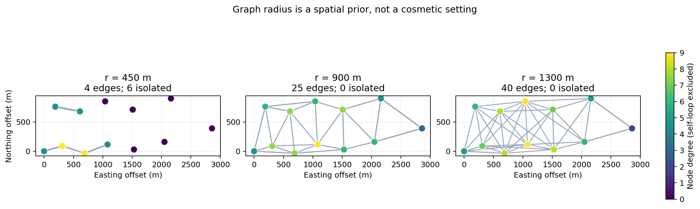
At 450 m, disconnected nodes cannot receive spatial context; at 900 m the survey is connected mainly through local neighbours; at 1300 m many long-range edges blur the meaning of locality. The middle value is not automatically correct—the appropriate radius must also survive held-out geology, coordinate perturbation, and response-space tests—but this view exposes topology that a validation-loss table would conceal.#
6.3.13.10. 9. Decide whether joint inversion is justified#
pycsamt.ai.inversion.JointInverter fuses two or more feature matrices
into one layered target:
>>> from pycsamt.ai.inversion import JointInverter
>>>
>>> joint = JointInverter(
...     n_features_list=(64, 25),
...     n_layers=5,
...     growth_rate=32,
...     n_dense_layers=6,
...     hidden_dim=256,
...     dropout=0.20,
...     log_thickness=True,
... )
>>> print(joint.__class__.__name__, joint.n_features_list, joint.n_layers)
JointInverter (64, 25) 5
Joint inversion is justified when modalities:
observe compatible locations and support volumes;
share a defensible common target or cross-property relationship;
are aligned without label leakage;
provide complementary rather than redundant information;
have realistic joint synthetic examples;
remain available under the deployment policy.
Compare against each modality alone. A fused network that improves aggregate loss may rely almost entirely on one modality or learn spurious correlations. Test missing-modality behavior explicitly.
Use an ablation study for joint models. Train or evaluate variants with one modality removed, shuffled, corrupted, or replaced by a baseline. If the joint model still performs well after a supposedly important modality is shuffled, the model is not using that modality in a scientifically meaningful way.
6.3.13.11. 10. Decide between supervised, PINN, and hybrid#
Choose supervised when#
a representative synthetic generator exists;
repeated low-latency inference is important;
target labels and parameterization are trustworthy;
domain coverage can be tested.
Choose PINN when#
labelled model generation is a bottleneck;
differentiable physics matches the observations;
per-survey optimization cost is acceptable;
data-fit and regularization need direct control;
convergence can be reviewed for every run.
Choose hybrid when#
an AI prior provides a useful initialization;
field response refinement is required;
supervised domain shift is a concern;
the extra two-stage complexity is justified by independent improvement.
Compare final response fit, structural stability, runtime, and failure rate. Do not compare supervised inference latency alone with a PINN’s complete optimization and conclude that the latter is inferior without considering the different task.
6.3.13.12. 11. Decide whether an ensemble is required#
pycsamt.ai.inversion.EnsembleInverter trains or combines compatible
base estimators.
Use an ensemble when:
uncertainty or stability is part of the decision;
member diversity can be created through seeds, data, or architectures;
calibration and test sets are large enough;
multiplied training and storage cost are acceptable.
Member disagreement measures only differences among members. If every member uses the same incorrect simulator or narrow prior, the ensemble can agree and still be wrong. Compare raw spread, calibrated coverage, interval sharpness, and field domain diagnostics.
6.3.13.13. 12. Establish baselines#
Every selection study should include:
- Simple statistical baseline
Mean target, nearest synthetic neighbor, or simple regression where appropriate. This reveals whether the network learns more than dataset bias.
- Simple neural baseline
Usually FCN or compact 1-D network.
- Dimensional baseline
Independent 1-D predictions before U-Net or graph context.
- Physics baseline
Forward reconstruction and a classical inversion appropriate to the survey, such as built-in 1-D, Occam2D, ModEM, or MARE2DEM.
- Operational baseline
Current project method, including runtime and reviewer effort.
A candidate should improve a declared criterion without unacceptable losses in calibration, robustness, interpretability, or deployability.
6.3.13.14. 13. Define a fair comparison protocol#
Hold constant across candidates:
dataset version and split indices;
feature and target transformations;
training and validation roles;
number of repeated seeds;
early-stopping policy;
optimization budget where comparable;
metric implementation;
test and field evaluation sets;
hardware or normalized resource accounting.
Architecture-specific tuning is legitimate, but the tuning budget should be comparable and documented. Report the distribution across repeated runs rather than only the best seed.
Use nested selection when possible:
inner validation chooses architecture and hyperparameters;
calibration fits uncertainty after model choice;
untouched synthetic test estimates final in-domain performance;
withheld field evidence assesses transfer.
Do not choose architecture, layer count, and reporting threshold on the same test observations.
6.3.13.15. 14. Compare multiple metric families#
- Model-space
Log-resistivity error, thickness error, boundary-depth error, section error, and performance by depth or geology.
- Response-space
Error-weighted impedance, apparent-resistivity, phase, or decay residuals after forward reconstruction.
- Structural
Conductor detection, boundary overlap, continuity, false targets, and edge behavior.
- Uncertainty
Coverage, interval width, reliability, ensemble spread, and failure under domain shift.
- Robustness
Noise, missing bands, station dropout, static shift, coordinate perturbation, and out-of-prior geology.
- Operational
Training time, inference time, peak memory, artifact size, persistence, backend availability, and reproducibility.
- Field
Classical response fit, borehole or geological agreement, and stability of the actual decision.
Aggregate averages can hide failure in deep layers, rare conductive targets, or sparse stations. Report distributions and scenario-stratified results.
When a scalar ranking is required, normalize each metric against an agreed reference before combining it. One defensible pattern is
In equation (11), \(M_c\) is a model-space error, \(R_c\) is a response-space error, \(U_c\) is an uncertainty penalty, \(T_c\) is runtime or resource cost, subscript \(b\) denotes the baseline, and \(P_c\) is a hard penalty for failing mandatory gates. Lower is better only if all quantities are defined that way.
>>> candidates = {
...     "fcn": {"model": 0.32, "response": 1.18, "uncertainty": 0.20, "runtime": 1.0, "gate": 0.0},
...     "resnet": {"model": 0.24, "response": 0.94, "uncertainty": 0.16, "runtime": 1.6, "gate": 0.0},
...     "unet2d": {"model": 0.22, "response": 0.91, "uncertainty": 0.28, "runtime": 3.4, "gate": 0.5},
... }
>>> baseline = candidates["fcn"]
>>> weights = {"model": 0.35, "response": 0.35, "uncertainty": 0.20, "runtime": 0.10}
>>> scores = {}
>>> for name, row in candidates.items():
...     score = row["gate"]
...     for metric, weight in weights.items():
...         score += weight * row[metric] / baseline[metric]
...     scores[name] = round(score, 3)
>>> scores
{'fcn': 1.0, 'resnet': 0.861, 'unet2d': 1.631}
>>> min(scores, key=scores.get)
'resnet'
The score does not replace scientific review. In this toy example, the 2-D candidate has strong model and response errors but receives a gate penalty, which might represent unresolved profile-width handling, failed dimensionality evidence, or unacceptable field residuals. Without that penalty, the ranking would silently ignore a deployment or validation failure.
More importantly, a single score hides run-to-run dispersion and weight sensitivity. The controlled illustration below uses explicit synthetic candidate metrics—it is a decision-analysis example, not a pyCSAMT benchmark. All costs are normalized to the FCN baseline, twelve seeded perturbations show why a mean is insufficient, and the dashed U-Net curve denotes a candidate that failed a mandatory gate.
View selection-trade-off source codeClick to inspect and copy the complete code
 1def make_model_selection_tradeoff() -> None:
 2    """Illustrate gates, Pareto trade-offs, and score-weight sensitivity."""
 3    names = np.array(["FCN", "CNN1D", "ResNet", "U-Net2D", "GCN"])
 4    metrics = np.array(
 5        [
 6            [1.00, 1.00, 1.00, 1.00],
 7            [0.91, 0.95, 0.93, 1.25],
 8            [0.76, 0.80, 0.78, 1.70],
 9            [0.69, 0.73, 1.31, 3.10],
10            [0.72, 0.76, 0.89, 2.45],
11        ]
12    )
13    gate_pass = np.array([True, True, True, False, True])
14    rng = np.random.default_rng(42)
15    seed_scores = np.clip(
16        metrics[:, 1, None] * rng.normal(1.0, 0.045, (5, 12)), 0, None
17    )
18
19    fig, axes = plt.subplots(1, 3, figsize=(13.2, 4.4))
20    ax_heat, ax_seed, ax_sensitivity = axes
21    image = ax_heat.imshow(metrics, cmap="YlGnBu_r", vmin=0.65, vmax=3.1)
22    ax_heat.set_xticks(range(4), ["model", "response", "calibration", "runtime"], rotation=28, ha="right")
23    ax_heat.set_yticks(range(5), names)
24    for i in range(5):
25        for j in range(4):
26            ax_heat.text(j, i, f"{metrics[i, j]:.2f}", ha="center", va="center", fontsize=8)
27    ax_heat.set_title("Baseline-normalized costs")
28    fig.colorbar(image, ax=ax_heat, shrink=0.75, label="lower is better")
29
30    parts = ax_seed.violinplot(seed_scores.T, showmeans=True, showextrema=False)
31    for body in parts["bodies"]:
32        body.set_facecolor("#60a5fa")
33        body.set_edgecolor("#1d4ed8")
34        body.set_alpha(0.68)
35    parts["cmeans"].set_color("#111827")
36    ax_seed.set_xticks(range(1, 6), names, rotation=28, ha="right")
37    ax_seed.set_ylabel("Response NRMS / FCN mean")
38    ax_seed.set_title("Twelve repeated-seed outcomes")
39    ax_seed.grid(axis="y", alpha=0.22)
40
41    response_weights = np.linspace(0.10, 0.70, 121)
42    fixed_calibration, fixed_runtime = 0.20, 0.10
43    for i, name in enumerate(names):
44        model_weights = 1.0 - response_weights - fixed_calibration - fixed_runtime
45        scores = (
46            model_weights * metrics[i, 0]
47            + response_weights * metrics[i, 1]
48            + fixed_calibration * metrics[i, 2]
49            + fixed_runtime * metrics[i, 3]
50        )
51        style = "--" if not gate_pass[i] else "-"
52        ax_sensitivity.plot(response_weights, scores, ls=style, lw=1.8, label=name)
53    ax_sensitivity.axvspan(0.10, 0.70, color="#f8fafc", zorder=-2)
54    ax_sensitivity.set(xlabel="Response-error weight", ylabel="Composite score")
55    ax_sensitivity.set_title("Scores depend on declared weights")
56    ax_sensitivity.grid(alpha=0.22)
57    ax_sensitivity.legend(frameon=False, fontsize=8, ncol=2)
58    fig.suptitle("A controlled selection illustration: evidence before one score")
59    fig.tight_layout()
60    _save(fig, "model_selection_tradeoff.png")
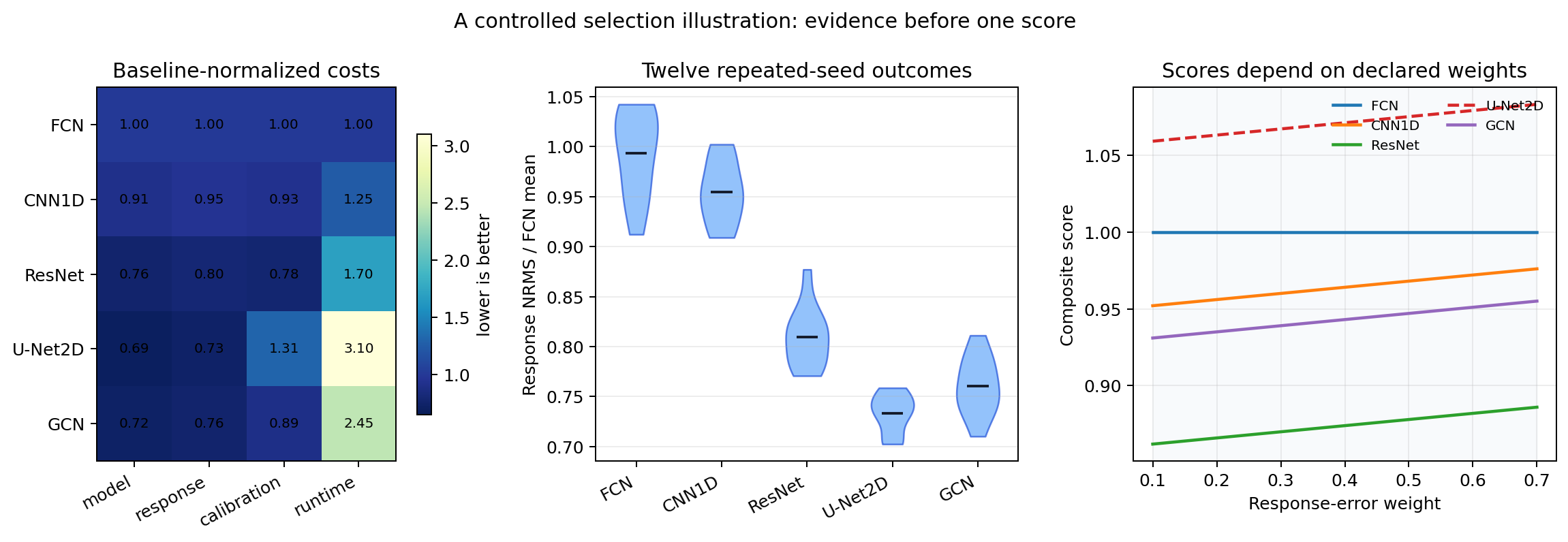
ResNet and GCN improve the model and response columns in this constructed study, but cost more to run; U-Net has low errors but fails its external gate and is therefore ineligible. The seed distributions overlap, so a small difference between means should not be treated as decisive. The right panel makes the governance issue visible: changing the declared response weight changes relative scores. Weights and gates must therefore be fixed before inspecting final test results, with the non-dominated alternatives retained when no stable winner exists.#
6.3.13.16. 15. Consider persistence and deployment#
The main supervised classes share public persistence support, but artifact contents and surrounding state still differ:
EMInverter1Dhas its specializedsave()/load()implementation;EMInverter2D,GCNInverter3D, andJointInverterinherit the public pair frompycsamt.ai.BaseEMNet;EnsembleInvertersaves and loads member checkpoints and ensemble metadata, but not attached uncertainty calibrators.
Availability of a method is not deployment evidence. Round-trip every final artifact in a clean target environment and compare predictions, normalization state, feature contract, graph construction, and software versions. A graph checkpoint, for example, does not make an unrecorded coordinate projection or radius reproducible.
Also evaluate:
CPU/GPU availability;
PyTorch or TensorFlow backend compatibility;
memory for profile/graph batch sizes;
offline or network restrictions;
checkpoint security and trusted loading;
latency and throughput;
monitoring and rollback requirements.
6.3.13.17. 16. Use InversionConfig for 1-D candidates#
pycsamt.ai.inversion.InversionConfig captures supported 1-D settings:
>>> from pycsamt.ai.inversion import InversionConfig
>>>
>>> config = InversionConfig(
...     arch="resnet",
...     n_layers=5,
...     solver="mt1d",
...     include_phase=True,
...     log_thickness=True,
...     augment_noise=0.02,
...     epochs=150,
...     batch_size=256,
...     lr=1e-3,
...     patience=20,
...     val_frac=0.15,
...     grad_clip=1.0,
...     seed=42,
...     checkpoint_dir="checkpoints",
...     checkpoint_name="mt1d_resnet_5l",
... )
>>> config.validate()
>>> inverter = config.to_inverter()
>>> fit_kwargs = config.to_fit_kwargs()
>>> print(config.arch, config.n_layers, fit_kwargs["epochs"], inverter.__class__.__name__)
resnet 5 150 EMInverter1D
>>> # Training needs a prepared dataset:
>>> # inverter.fit(dataset, **fit_kwargs)
validate() checks supported architecture, solver, device, and numerical
ranges. It does not evaluate scientific suitability.
weight_decay and min_delta are stored in the configuration for
documentation but are not currently included by to_fit_kwargs() because
EMInverter1D.fit does not expose them. Do not assume every configuration
field affects training. Likewise, save_best, checkpoint_dir, and
checkpoint_name do not make to_inverter() or to_fit_kwargs() save
automatically. The caller must save the fitted inverter explicitly. Calling
checkpoint_path() resolves the configured filename and creates its parent
directory, so use it only when that filesystem side effect is intended:
>>> path = config.checkpoint_path()
>>> path.as_posix().endswith("checkpoints/mt1d_resnet_5l.npz")
True
>>> # After fitting and acceptance testing:
>>> # inverter.save(path)
from_inverter() reconstructs architectural fields that are present on an
inverter; it cannot recover a past optimizer schedule or split policy that the
inverter does not retain. Preserve the original configuration and selection
record beside the checkpoint.
6.3.13.18. 17. Record the selection decision#
A model-selection record should contain:
model_selection/
├── selection_plan.yml
├── dataset_reference.yml
├── split_indices.npz
├── candidates.csv
├── metrics_by_seed.csv
├── metrics_by_scenario.csv
├── compute_profile.csv
├── rejected_candidates.md
├── selected_model.yml
└── review_signoff.md
For every candidate record:
family, dimension, architecture, and parameter count;
feature and target contract IDs;
training configuration and seeds;
validation/calibration/test metrics;
response reconstruction results;
domain-shift and robustness tests;
runtime, memory, artifact size, and persistence method;
known limitations and failure cases;
selection status and reason.
6.3.13.19. Complete selection example#
The following skeleton runs supported 1-D architectures repeatedly on one
dataset. Because the current fit(..., seed=...) uses the seed for its
internal train/validation split as well as training randomness, these runs
measure combined split-and-training sensitivity rather than a strictly fixed
split comparison. A controlled study should supply pre-separated arrays or a
project harness with frozen indices. Final selection must use project metrics,
not only the validation score stored by the inverter:
>>> from pycsamt.ai.inversion import InversionConfig
>>>
>>> planned = []
>>> for arch in ("fcn", "cnn1d", "resnet"):
...     for seed in (11, 22, 33):
...         cfg = InversionConfig(
...             arch=arch,
...             n_layers=5,
...             solver="mt1d",
...             include_phase=True,
...             epochs=100,
...             batch_size=256,
...             lr=1e-3,
...             patience=15,
...             val_frac=0.15,
...             seed=seed,
...             checkpoint_dir=None,
...             verbose=False,
...         )
...         cfg.validate()
...         planned.append((cfg.arch, cfg.seed, cfg.to_fit_kwargs()["epochs"]))
>>> len(planned)
9
>>> planned[:3]
[('fcn', 11, 100), ('fcn', 22, 100), ('fcn', 33, 100)]
>>> # In a real study, train each candidate on a prepared dataset:
>>> # model = cfg.to_inverter()
>>> # model.fit(dataset, **cfg.to_fit_kwargs())
This example only builds and validates the candidate grid. Production selection should then train each candidate on prepared data, write stable public histories or independently computed metrics, and never make a decision solely from private internals.
6.3.13.20. Selection checklist#
Check |
Evidence |
|---|---|
Objective declared first |
Primary metric, constraints, failure conditions, and decision tolerance. |
Dimension is geophysical |
Survey layout, strike, tensor/tipper diagnostics, and target geometry. |
Parameterization is resolvable |
Layer/depth tests, bandwidth, sensitivity, and boundary stability. |
Candidates are meaningful |
Simple baseline, supervised/PINN/hybrid rationale, and architecture assumptions. |
Comparison is fair |
Frozen data and splits, comparable tuning budget, repeated seeds, and untouched test set. |
Metrics are multidimensional |
Model, response, structure, uncertainty, robustness, field, and compute. |
Domain shift is tested |
Missingness, noise, nuisance effects, geology, geometry, and field coverage. |
Deployment is feasible |
Persistence, backend, hardware, security, latency, and rollback. |
Decision is auditable |
All candidates, rejected alternatives, declared selection rule, reviewer, and signoff. |
6.3.13.21. Common mistakes#
Avoid these errors:
choosing dimension from architecture availability rather than geophysics;
selecting the most complex model by default;
comparing candidates trained on different random splits;
tuning on the test or field-validation set;
reporting only the best seed;
increasing output depth cells and claiming improved physical resolution;
using variable-layer NaN targets without a mask-aware strategy;
confusing U-Net continuity with 2-D forward physics;
using identity adjacency and describing the result as spatial GCN inversion;
selecting graph radius without inspecting connectivity;
fusing modalities without testing each modality alone;
interpreting ensemble agreement as absence of shared bias;
comparing only validation loss and ignoring response reconstruction;
selecting a model that cannot be restored in production;
assuming every
InversionConfigfield is used byto_fit_kwargs().
6.3.13.22. Next steps#
Continue with:
Training AI inversion models to fit the selected candidate reproducibly;
AI inversion validation to run the final acceptance protocol;
AI inversion inference to deploy the approved model contract;
AI inversion uncertainty to select and calibrate predictive intervals;
Hybrid AI and physics inversion for AI warm-start plus physics refinement choices;
Physics-informed 2-D inversion for detailed physics-informed profile choices;
AI inversion reporting for the model-selection record and model card.
The WILLY dimensionality figure is reproduced by
docs/scripts/generate_ai_inversion_figures.py from the bundled L18 EDI
files. It is a deterministic diagnostic of the documented classification
rule, not an AI prediction or an accepted inversion model.