
6.3.19. Physics-informed 2-D inversion#
pycsamt.ai.inversion.PINNInverter2D is a
physics-informed inversion workflow that jointly optimizes layered
models for all stations on a profile. It uses a differentiable 1-D MT
forward operator at each station and couples adjacent station models
with lateral smoothness. The result is a pseudo-2-D resistivity section: a set
of jointly regularized 1-D models, not a full finite-element or
finite-difference 2-D EM forward inversion.
This distinction is central to scientific use. The workflow can provide a useful profile estimate when locally layered physics and lateral smoothness are reasonable approximations. It should not be presented as equivalent to Occam2D, MARE2DEM, ModEM, or another solver that explicitly models 2-D/3-D EM fields.
Meaning of “2-D”
“2-D” here describes the jointly optimized station–layer section and its lateral regularization. Data fit is calculated with the differentiable Wait-style MT 1-D recursion independently at each station. Strong lateral induction, off-profile structure, anisotropy, topography, and other missing physics can therefore produce a smooth but biased section.
6.3.19.1. When to use this workflow#
Consider PINN 2-D when:
stations form an ordered survey profile;
dimensionality evidence suggests locally 1-D or gently varying 2-D structure, with phase tensor and strike diagnostics reviewed;
a common layered parameterization is scientifically acceptable as a model prior;
no labelled model dataset is available or desired;
direct response-space optimization is preferred to supervised prediction;
a fast pseudo-2-D baseline or starting model is useful;
the result will be compared with classical inversion, response reconstruction, and independent data.
Prefer a full 2-D or 3-D classical solver when:
lateral induction is important to the target;
strong contacts, topography, coast effects, anisotropy, or 3-D structure are expected;
tensor components cannot be represented by per-station 1-D responses;
model appraisal requires the corresponding numerical forward physics;
regulatory or project standards require a recognized 2-D/3-D solver.
6.3.19.2. Workflow#
QC and order the profile data;
review strike and dimensionality evidence;
choose TE, TM, or the current averaged
bothmode;define the common frequency grid and supported depth;
choose layer count, smoothness weights, optimizer, and epochs;
run baseline and sensitivity configurations;
inspect convergence and response-space metric residuals;
compare section, thicknesses, and reconstructed responses across scenarios;
validate against classical inversion and independent evidence;
report the pseudo-2-D physics and all limitations explicitly.
6.3.19.3. 1. Understand the model parameterization#
For S stations and L layers, the optimizer uses:
log_rho.shape   = (S, L)
log_thick.shape = (S, L - 1)
Both arrays are optimized jointly. Resistivity is represented as \(\log_{10}(\rho/\Omega\mathrm{m})\); thickness is represented internally in log10 metres and converted back for output.
The optimized station model is therefore
where \(u_{s\ell}=\log_{10}\rho_{s\ell}\) and \(q_{s\ell}=\log_{10}h_{s\ell}\). The pseudo-2-D section is the matrix \(U=[u_{s\ell}]\), but the forward response at station \(s\) still depends only on \(\mathbf{m}_s\). Lateral coupling enters through regularization, not through a 2-D electromagnetic field calculation.
The public section methods transpose the internal station-major layout:
resistivity_section.shape = (L, S)
thickness_section.shape   = (L - 1, S)
Each station has its own interface thicknesses. Consequently, layer index is a parameter correspondence, not automatically a continuous geological horizon. Inspect cumulative interface depths before drawing boundaries between stations.
For each station, cumulative interface depth is
If thickness varies laterally, the same layer index can sit at different physical depths from station to station. Plotting only layer index is useful for debugging, but it is not a physical-depth interpretation.
depth_max guides the layered depth parameterization and initialization; it
does not establish a geophysical depth of investigation. The defensible
interpretation depth must come from bandwidth, sensitivity, response fit, and
scenario stability.
The physics enters through a differentiable Wait recursion. For angular frequency \(\omega=2\pi f\), magnetic permeability \(\mu_0\), and layer \(\ell\), define the propagation constant and intrinsic impedance
Starting in the basement with \(Z_L=\eta_L\), the implementation moves upward through each finite layer:
The surface impedance gives the predicted observables
Equations (3) through (5) are evaluated for all stations as one differentiable batch. Automatic differentiation therefore supplies gradients with respect to both \(u_{s\ell}\) and \(q_{s\ell}\). The batch dimension improves execution efficiency; it does not couple electromagnetic fields between stations. Only \(\mathcal R_x\) supplies lateral coupling.
6.3.19.4. 2. Understand the loss function#
The implemented objective combines data fit, vertical smoothing, and lateral smoothing:
Data term#
For valid station–frequency cells, the data term combines squared differences in log10 apparent resistivity and normalized phase:
N_v is the number of finite observations after common-grid interpolation.
Missing cells are excluded from the data term.
Equivalently, with finite-data mask \(M_{sf}\),
A station with fewer valid frequencies contributes fewer residual terms. It may still look smooth in the final section because lateral regularization borrows structure from neighboring stations. Inspect valid-cell counts before interpreting weakly constrained stations.
The 90-degree phase normalization makes the two residual blocks numerically comparable but is not an observational covariance model. Formal errors and station-specific uncertainty are not explicit weights in this objective.
If project errors are available, compare the final section with an external normalized RMS misfit calculation in AI inversion validation. The optimizer loss and a formal error-weighted inversion RMS are related diagnostics, not the same statistic.
Vertical regularization#
smoothness_weight is \(\lambda_z\). It penalizes changes in log
resistivity between adjacent layers at each station. Larger values favor
vertically smooth models; smaller values permit sharper changes and greater
instability.
In station-layer notation, a representative vertical penalty is
Lateral regularization#
lateral_weight is \(\lambda_x\). It penalizes log-resistivity
differences between adjacent stations at the same layer index. It assumes the
input station order represents profile adjacency.
The corresponding chain penalty is
The lateral term does not currently scale differences by physical station spacing. Closely and widely spaced station pairs are treated as adjacent indices. Resample carefully or interpret regularization strength in light of irregular chainage.
Thickness regularization and constraints#
Resistivity smoothness is explicit in the documented objective. Layer thicknesses are optimized in log space, but the same lateral/vertical regularization description should not be assumed to apply to them unless confirmed in the backend kernel. Audit thickness stability separately.
The backend confirms two further details. Thickness is not included in either
roughness term, and after every optimizer update its log10 value is clipped to
[0, 5]. Thus each finite-layer thickness is constrained to
\(1\le h\le100{,}000\) m. Resistivity has no analogous explicit clamp.
These are numerical constraints, not geological bounds; project-specific
plausibility still needs an external acceptance check.
6.3.19.5. 3. Prepare and order profile data#
Load the profile canonically and verify station order before constructing the inverter:
>>> from pycsamt.emtools import ensure_sites
>>>
>>> sites = ensure_sites(
...     "data/AMT/WILLY_data/L18PLT",
...     recursive=True,
...     verbose=0,
... )
The public observation bridge can then be inspected without starting an optimizer. On the bundled line it produces 28 station records with aligned TE and TM arrays at each station:
>>> from pycsamt.ai.inversion import sites_to_obs_2d
>>> observations = sites_to_obs_2d(
...     "data/AMT/WILLY_data/L18PLT", verbose=0
... )
>>> len(observations)
28
>>> first = observations[0]
>>> first.name, first.freq.shape, first.rho_te.shape, first.rho_tm.shape
('18-001A', (53,), (53,), (53,))
>>> coverage = (
...     min(float(item.freq.min()) for item in observations),
...     max(float(item.freq.max()) for item in observations),
... )
>>> coverage
(1.008, 10400.0)
The inverter uses pycsamt.ai.inversion.sites_to_obs_2d() internally and
preserves the order returned by the input. It does not sort stations by
chainage. Provide a Sites object already ordered along
the intended profile direction.
Retain a table containing:
station name;
profile distance in metres;
easting, northing, and elevation;
original and inversion order;
valid frequency range;
TE/TM component completeness;
QC exclusions and corrections.
Do not infer physical x coordinates from array column number in a final plot.
6.3.19.6. 4. Select polarization mode#
mode accepts "te", "tm", or "both".
teUses the component named by
comp_te, default"xy".tmUses the component named by
comp_tm, default"yx". The public observation bridge stores TM phase as magnitude.bothIn the current implementation, averages TE and TM apparent resistivity and averages TE and TM phase before optimization. It does not form two independent data-misfit blocks or jointly fit both modes separately.
Warning
Averaging TE and TM can suppress genuine mode differences caused by 2-D/3-D
structure. Use mode="both" only as an explicitly reviewed approximation.
For scientific comparison, run TE and TM separately and inspect their
disagreement.
Mode labels depend on profile orientation and strike convention. Verify these before accepting the defaults.
6.3.19.7. 5. Choose the common frequency grid#
The constructor extracts valid observations and builds a log-spaced common
grid with n_freqs points spanning the combined available range:
>>> from pycsamt.ai.inversion import PINNInverter2D
>>>
>>> inversion = PINNInverter2D(
...     sites,
...     n_layers=10,
...     depth_max=2000.0,
...     n_freqs=32,
...     mode="te",
... )
Each station is interpolated to this grid in log-frequency space. Values outside a station’s own range become NaN and do not contribute to the data loss.
Because the public constructor does not expose explicit freq_min and
freq_max arguments, the common endpoints follow the extracted survey
coverage. To enforce a project-specific range, prefilter the reviewed data or
extend the API through a tested project change rather than mutating private
attributes.
Inspect coverage per station. A station constrained by only a small subset of the common grid can borrow visual smoothness from neighbors without having the same depth sensitivity.
The public pycsamt.ai.inversion.sites_to_obs_2d() bridge makes the
pre-fit inspection reproducible. The following code extracts the actual WILLY
L18 TE/TM arrays, constructs a display grid without extrapolation, and compares
mode support and disagreement before any model is optimized.
View PINN 2-D input-diagnostic source codeClick to inspect and copy the complete code
 1def make_pinn2d_input_diagnostic() -> None:
 2    """Inspect WILLY frequency support and TE/TM disagreement before fitting."""
 3    line = PROJECT_ROOT / "data" / "AMT" / "WILLY_data" / "L18PLT"
 4    observations = sites_to_obs_2d(line, comp_te="xy", comp_tm="yx")
 5    frequency = np.logspace(
 6        np.log10(min(o.freq.min() for o in observations)),
 7        np.log10(max(o.freq.max() for o in observations)),
 8        48,
 9    )
10
11    def interpolate(obs, values):
12        order = np.argsort(obs.freq)
13        result = np.interp(
14            np.log10(frequency), np.log10(obs.freq[order]), values[order]
15        )
16        outside = ((frequency < obs.freq.min() * (1.0 - 1e-12)) |
17                   (frequency > obs.freq.max() * (1.0 + 1e-12)))
18        result[outside] = np.nan
19        return result
20
21    te_rho = np.vstack(
22        [interpolate(o, np.log10(o.rho_te)) for o in observations]
23    )
24    tm_rho = np.vstack(
25        [interpolate(o, np.log10(o.rho_tm)) for o in observations]
26    )
27    te_phase = np.vstack([interpolate(o, o.phase_te) for o in observations])
28    tm_phase = np.vstack([interpolate(o, o.phase_tm) for o in observations])
29    valid = np.isfinite(te_rho) & np.isfinite(te_phase)
30
31    fig, axes = plt.subplots(2, 2, figsize=(12.2, 8.0))
32    ax_coverage, ax_rho, ax_phase, ax_count = axes.ravel()
33    coverage = ax_coverage.pcolormesh(
34        frequency, np.arange(len(observations)), valid,
35        cmap="Blues", shading="nearest", vmin=0, vmax=1,
36    )
37    ax_coverage.set_xscale("log")
38    ax_coverage.set(
39        xlabel="Frequency (Hz)", ylabel="Station index",
40        title="Common-grid support (blue = valid)",
41    )
42
43    ax_rho.plot(
44        frequency, np.nanmedian(te_rho, axis=0), color="#2563eb",
45        lw=2, label="TE / xy",
46    )
47    ax_rho.plot(
48        frequency, np.nanmedian(tm_rho, axis=0), color="#f15a29",
49        lw=2, label="TM / |yx|",
50    )
51    ax_rho.set_xscale("log")
52    ax_rho.set(
53        xlabel="Frequency (Hz)", ylabel=r"Median $\log_{10}\rho_a$",
54        title="Modes are not interchangeable",
55    )
56    ax_rho.grid(alpha=0.22, which="both")
57    ax_rho.legend(frameon=False)
58
59    phase_difference = te_phase - tm_phase
60    phase_image = ax_phase.pcolormesh(
61        frequency, np.arange(len(observations)),
62        phase_difference, cmap="coolwarm", shading="nearest", vmin=-180, vmax=180,
63    )
64    ax_phase.set_xscale("log")
65    ax_phase.set(
66        xlabel="Frequency (Hz)", ylabel="Station index",
67        title="TE minus TM phase (degrees)",
68    )
69    fig.colorbar(phase_image, ax=ax_phase, shrink=0.86, label="Phase difference (°)")
70
71    phase_rms = np.sqrt(np.nanmean(phase_difference**2, axis=1))
72    rho_rms = np.sqrt(np.nanmean((te_rho - tm_rho) ** 2, axis=1))
73    station_index = np.arange(len(observations))
74    ax_count.bar(station_index, phase_rms, color="#3e65b0", alpha=0.78)
75    ax_count.set(
76        xlabel="Station index", ylabel="TE–TM phase RMS (degrees)",
77        title="Mode disagreement by station",
78    )
79    ax_rho_rms = ax_count.twinx()
80    ax_rho_rms.plot(station_index, rho_rms, color="#f15a29", marker="o", ms=3)
81    ax_rho_rms.set_ylabel(r"TE–TM $\log_{10}\rho_a$ RMS", color="#f15a29")
82    ax_count.grid(axis="y", alpha=0.22)
83    fig.suptitle("WILLY L18 inputs to PINNInverter2D — inspect before optimization")
84    fig.tight_layout()
85    _save(fig, "pinn2d_input_diagnostic.png")
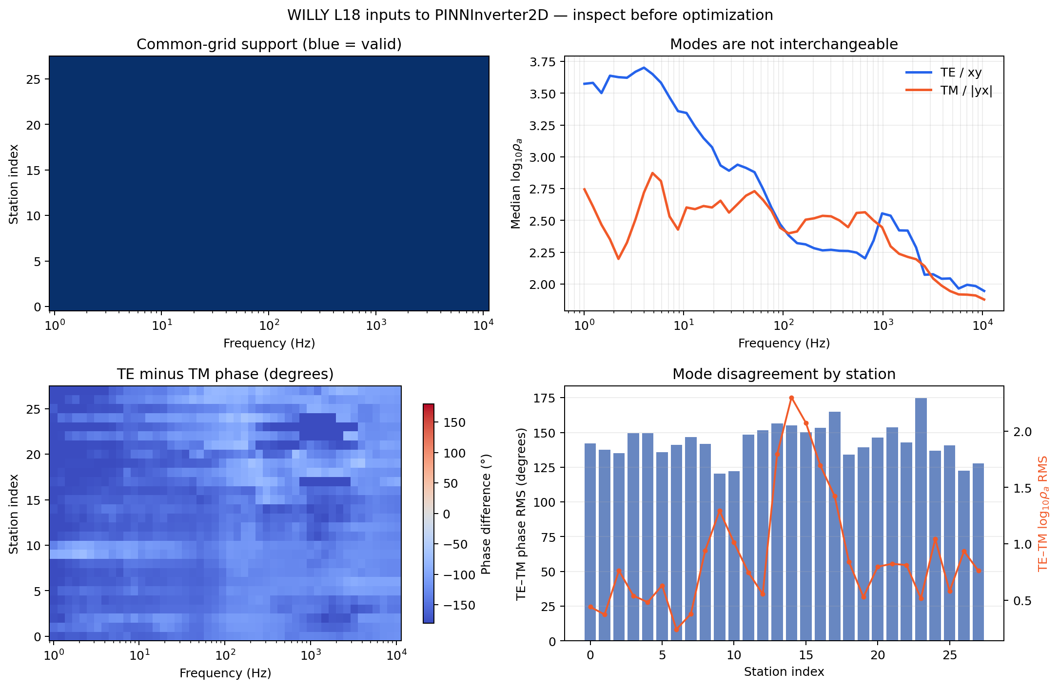
WILLY stations cover almost the same displayed frequency range, so the common-grid mask alone looks reassuring. The mode panels tell a different story: TE and TM apparent resistivity separate strongly over important bands, and the phase convention creates large systematic differences. Averaging these modes would erase evidence rather than resolve it. Separate TE and TM runs, dimensionality review, and component-aware residuals are required before choosing a preferred section.#
6.3.19.8. 6. Choose layer count and depth#
Start with the simplest parameterization able to represent expected electrical units. Test several defensible combinations, for example:
>>> candidates = [
...     {"n_layers": 6, "depth_max": 1500.0},
...     {"n_layers": 10, "depth_max": 2000.0},
...     {"n_layers": 14, "depth_max": 3000.0},
... ]
>>> len(candidates)
3
>>> candidates[1]
{'n_layers': 10, 'depth_max': 2000.0}
Increasing layers can reduce response residuals while adding unstable
interfaces. Increasing depth_max can allocate parameters below meaningful
sensitivity. Compare:
reconstructed response fit;
interface-depth stability;
deep-layer variation across runs;
dependence on smoothing;
classical inversion and sensitivity depth;
independent borehole or geological evidence.
Do not interpret the bottom of the configured model as the investigation depth.
6.3.19.9. 7. Select regularization weights#
The defaults are:
smoothness_weight = 0.01
lateral_weight    = 0.005
Treat them as starting values, not universal choices. Run a grid of plausible weights:
>>> scenarios = [
...     (0.001, 0.0005),
...     (0.01, 0.005),
...     (0.05, 0.02),
... ]
>>> len(scenarios)
3
>>> scenarios[0]
(0.001, 0.0005)
For each scenario, retain total loss, response residuals, roughness measures, section differences, and target stability. The reported convergence curve contains total loss, not separate data and regularization histories, so additional diagnostics may require calculation from outputs or backend instrumentation.
Avoid choosing weights solely for a visually smooth section. Excessive lateral smoothing can smear faults, isolated conductors, or station-specific problems. Insufficient smoothing can fit noise with alternating layers.
The next controlled example isolates the geometry of the two penalties. It solves a quadratic denoising analogue with the same vertical and lateral first-difference operators; it does not claim to be an electromagnetic inversion benchmark. That separation is useful because it shows what each regularizer is capable of suppressing before forward-physics complexity is introduced.
View regularization-anatomy source codeClick to inspect and copy the complete code
 1def make_pinn2d_regularization_anatomy() -> None:
 2    """Visualize the separate effects of vertical and lateral roughness."""
 3    stations, layers = 30, 12
 4    x = np.linspace(0, 1, stations)
 5    truth = np.full((stations, layers), 2.5)
 6    truth[:, :3] = 2.0
 7    truth[(x > 0.28) & (x < 0.68), 4:8] = 0.8
 8    truth[x > 0.76, 6:10] = 3.5
 9    rng = np.random.default_rng(27)
10    proxy = truth + rng.normal(0, 0.42, truth.shape)
11
12    dz = np.eye(layers, k=1) - np.eye(layers)
13    dz = dz[:-1]
14    dx = np.eye(stations, k=1) - np.eye(stations)
15    dx = dx[:-1]
16    identity = np.eye(stations * layers)
17    pz = np.kron(np.eye(stations), dz.T @ dz)
18    px = np.kron(dx.T @ dx, np.eye(layers))
19
20    settings = [(0.0, 0.0), (3.0, 0.0), (0.0, 3.0), (1.2, 1.2)]
21    estimates = []
22    diagnostics = []
23    vector = proxy.ravel()
24    for lam_z, lam_x in settings:
25        estimate = np.linalg.solve(identity + lam_z * pz + lam_x * px, vector)
26        estimate = estimate.reshape(stations, layers)
27        estimates.append(estimate)
28        data = np.mean((estimate - proxy) ** 2)
29        vertical = np.mean(np.diff(estimate, axis=1) ** 2)
30        lateral = np.mean(np.diff(estimate, axis=0) ** 2)
31        diagnostics.append((data, vertical + lateral))
32
33    fig, axes = plt.subplots(2, 3, figsize=(12.8, 7.7))
34    panels = [truth, proxy, estimates[1], estimates[2], estimates[3]]
35    titles = [
36        "Known log-resistivity", "Noisy data-fit proxy",
37        r"Vertical only: $\lambda_z=3$", r"Lateral only: $\lambda_x=3$",
38        r"Balanced: $\lambda_z=\lambda_x=1.2$",
39    ]
40    for ax, values, title in zip(axes.ravel()[:5], panels, titles):
41        image = ax.imshow(
42            values.T, origin="upper", aspect="auto", cmap="turbo",
43            vmin=0.5, vmax=3.8,
44        )
45        ax.set(title=title, xlabel="Station index", ylabel="Layer index")
46
47    ax_trade = axes.ravel()[5]
48    for (data, roughness), (lam_z, lam_x) in zip(diagnostics, settings):
49        ax_trade.scatter(data, roughness, s=65)
50        ax_trade.annotate(
51            f"({lam_z:g}, {lam_x:g})", (data, roughness),
52            xytext=(5, 5), textcoords="offset points", fontsize=8,
53        )
54    ax_trade.set(
55        xlabel="Data-proxy MSE", ylabel="Vertical + lateral roughness",
56        title=r"Trade-off labels: $(\lambda_z,\lambda_x)$",
57    )
58    ax_trade.grid(alpha=0.22)
59    color_axis = fig.add_axes([0.92, 0.18, 0.012, 0.64])
60    fig.colorbar(image, cax=color_axis, label=r"$\log_{10}\rho$ ($\Omega$ m)")
61    fig.suptitle("Regularization changes what the pseudo-2-D model is allowed to express")
62    fig.subplots_adjust(left=0.07, right=0.89, bottom=0.09, top=0.88, hspace=0.36, wspace=0.30)
63    _save(fig, "pinn2d_regularization_anatomy.png")
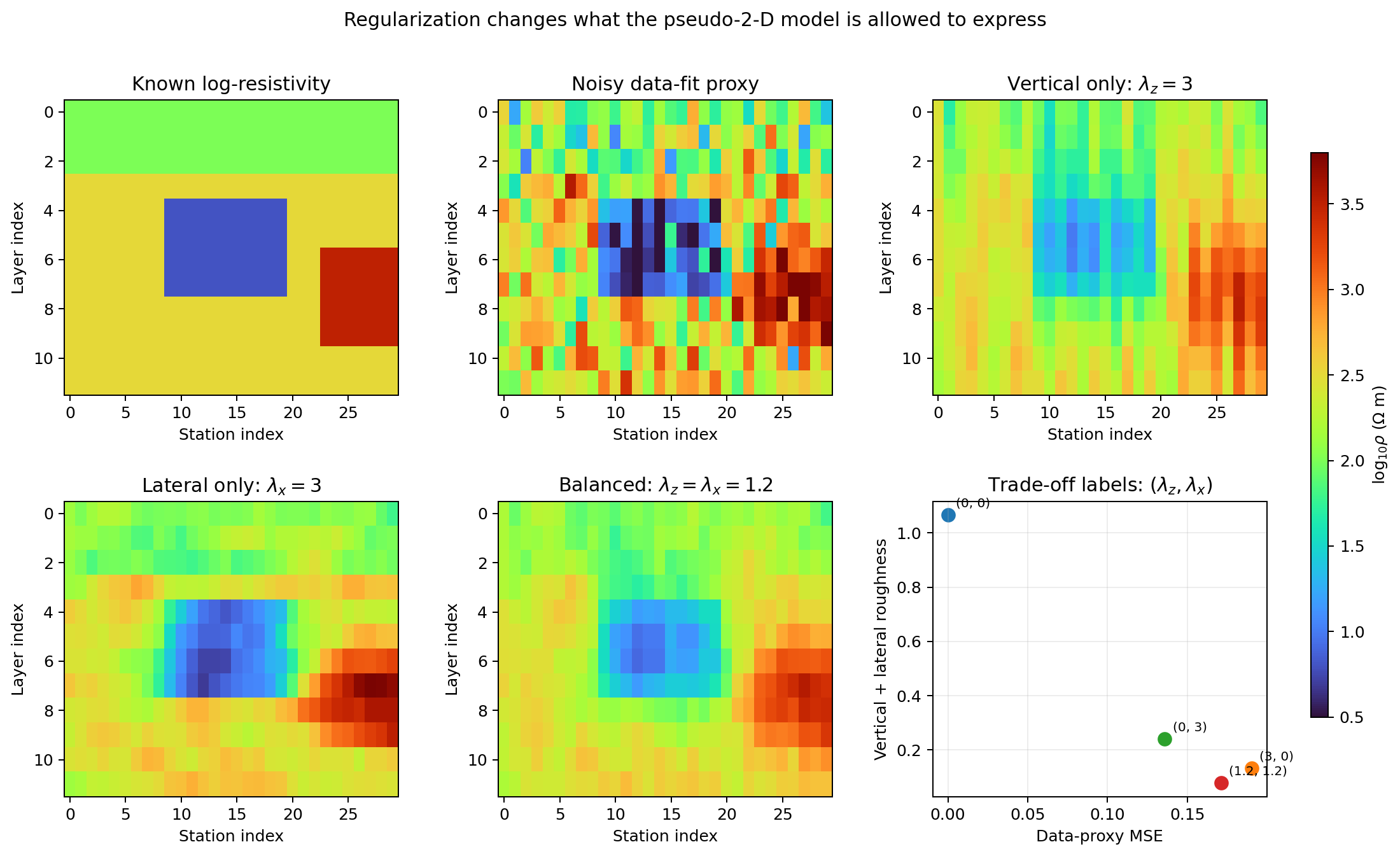
Vertical smoothing blends layer boundaries within each station but leaves lateral noise; lateral smoothing preserves sharper vertical changes while spreading anomalies along the profile. Balanced smoothing suppresses both kinds of roughness but rounds the known conductor and resistor boundaries. The trade-off panel confirms that roughness reduction is purchased with departure from the data-fit proxy. In a real inversion the selected point must also pass response reconstruction and target-stability tests.#
6.3.19.10. 8. Select optimizer controls#
epochsMaximum Adam iterations, default 300.
lrAdam learning rate, default
1e-2.devicePyTorch/TensorFlow device resolved through the active backend.
The current high-level fit() does not expose early stopping, validation
data, or learning-rate scheduling. Gradient clipping is active inside both
backends at norm 5, but its threshold is not a public option. The implementation
runs the requested optimization iterations through the backend kernel. Monitor
the curve and run repeat configurations rather than assuming the final epoch
is optimal.
Unless a hybrid workflow supplies an initial model to the lower-level kernel, all stations and layers start at the global mean observed \(\log_{10}\rho_a\); each finite thickness starts at \(\max(d_{max}/L,1)\) m. This laterally uniform initialization is another prior. Repeated runs from the same inputs are not a meaningful initialization ensemble unless initialization is deliberately changed through a supported workflow.
A large learning rate can oscillate or diverge; a very small rate may appear stable without reaching an adequate fit. Compare final sections across epochs and learning rates.
6.3.19.11. 9. Run a baseline inversion#
>>> from pycsamt.ai.inversion import PINNInverter2D
>>>
>>> inversion = PINNInverter2D(
...     sites,
...     n_layers=10,
...     depth_max=2000.0,
...     n_freqs=32,
...     mode="te",
...     smoothness_weight=0.01,
...     lateral_weight=0.005,
...     epochs=300,
...     lr=1e-2,
...     comp_te="xy",
...     comp_tm="yx",
...     device=None,
...     verbose=0,
... )
>>> inversion.fit(verbose=True, log_every=25)
>>> print(inversion)
>>> print(inversion.stations)
>>> print(inversion.n_sites)
The constructor performs data extraction immediately and can raise before
fit() when no valid observations survive. The deep-learning backend is
required when fitting.
Executed WILLY smoke test#
The documentation generator executed a deliberately short CPU run on the 28
EDI files in data/AMT/WILLY_data/L18PLT using eight layers, 24 common
frequencies, TE/xy, 2 km configured depth, 20 epochs, and the constructor’s
default-scale learning rate of \(10^{-2}\). The captured audit is:
stations=28
section_shape=(8, 28)
thickness_shape=(7, 28)
loss_first=0.955507
loss_final=1.788527
minimum_loss=0.955507 at epoch 1
log10_apparent_resistivity_RMSE=0.805332
phase_RMSE_deg=40.579903
finite_residual_rows=1484 of 1484
This run fails the convergence gate: its final objective is 87.2% larger than
the first recorded value, and the minimum occurs at epoch 1. Smaller smoke-test
learning rates of 3e-3 and 1e-3 also failed to improve the first loss.
The resulting colors must therefore not be interpreted as WILLY geology. They
are retained below because a failed run is useful for demonstrating both the
required diagnostic and the topographic display transformation.
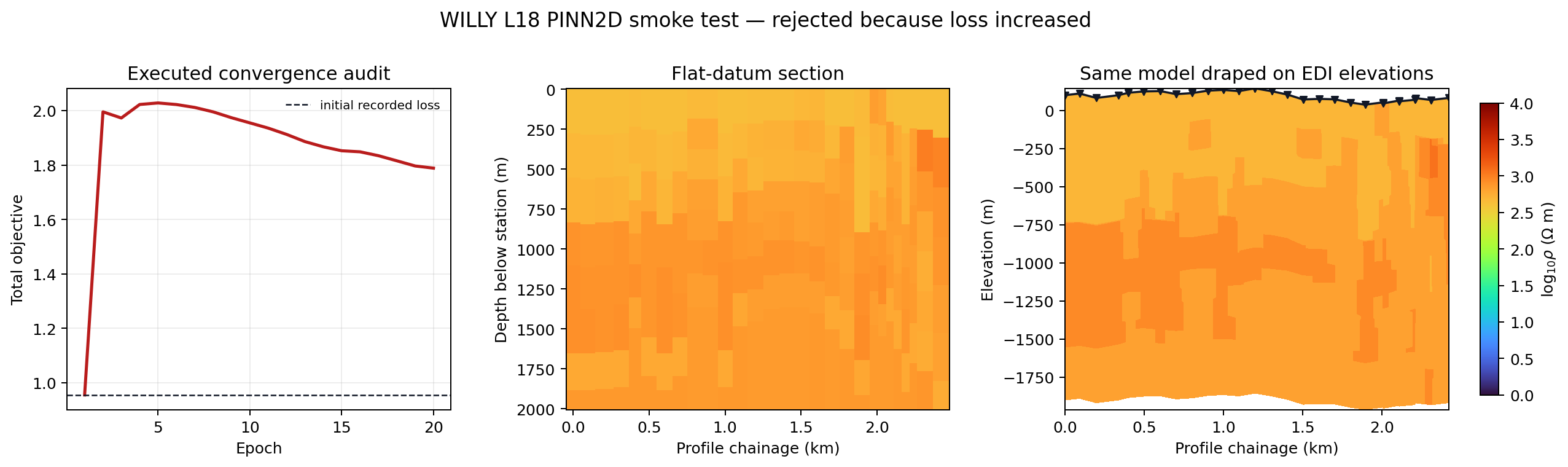
Executed WILLY L18 smoke-test audit. The middle and right panels contain the same resistivity values; only their vertical coordinates differ. The title records the rejection so that the terrain rendering cannot be mistaken for a validated inversion result.#
The complete executed plotting and audit code is available without interrupting the interpretation flow:
View executed WILLY PINN 2-D audit source codeClick to inspect and copy the complete code
  1def make_pinn2d_willy_topography_audit() -> None:
  2    """Execute and display a deliberately short, auditable WILLY PINN run."""
  3    try:
  4        import torch
  5
  6        torch.manual_seed(241)
  7    except ImportError:
  8        pass
  9    np.random.seed(241)
 10    line = PROJECT_ROOT / "data" / "AMT" / "WILLY_data" / "L18PLT"
 11    sites = ensure_sites(line, recursive=True, verbose=0)
 12    inverter = PINNInverter2D(
 13        line,
 14        n_layers=8,
 15        depth_max=2000.0,
 16        n_freqs=24,
 17        mode="te",
 18        smoothness_weight=0.01,
 19        lateral_weight=0.005,
 20        epochs=20,
 21        lr=1e-2,
 22        device="cpu",
 23        verbose=0,
 24    ).fit(verbose=False)
 25    loss = inverter.convergence_curve()["loss"].to_numpy()
 26    section = inverter.resistivity_section(as_log10=True)
 27    thickness = inverter.thickness_section()
 28
 29    station_list = list(sites)
 30    latitude = np.array([site.coords[0] for site in station_list], dtype=float)
 31    longitude = np.array(
 32        [site.coords[1] for site in station_list], dtype=float
 33    )
 34    elevation = np.array(
 35        [site.coords[2] for site in station_list], dtype=float
 36    )
 37    radius = 6_371_000.0
 38    lat_rad = np.deg2rad(latitude)
 39    lon_rad = np.deg2rad(longitude)
 40    dlat = np.diff(lat_rad)
 41    dlon = np.diff(lon_rad)
 42    hav = np.sin(dlat / 2) ** 2 + (
 43        np.cos(lat_rad[:-1]) * np.cos(lat_rad[1:]) * np.sin(dlon / 2) ** 2
 44    )
 45    segment = 2 * radius * np.arcsin(np.sqrt(np.clip(hav, 0, 1)))
 46    chainage = np.r_[0.0, np.cumsum(segment)] / 1000.0
 47
 48    depth = np.linspace(0.0, 2000.0, 201)
 49    resampled = np.empty((len(depth), section.shape[1]))
 50    for station in range(section.shape[1]):
 51        interfaces = np.cumsum(thickness[:, station])
 52        layer = np.searchsorted(interfaces, depth, side="right")
 53        layer = np.clip(layer, 0, section.shape[0] - 1)
 54        resampled[:, station] = section[layer, station]
 55
 56    fig, axes = plt.subplots(1, 3, figsize=(14.2, 4.4))
 57    axes[0].plot(np.arange(1, len(loss) + 1), loss, color="#b91c1c", lw=2)
 58    axes[0].axhline(
 59        loss[0], color="#111827", ls="--", lw=1, label="initial recorded loss"
 60    )
 61    axes[0].set(
 62        xlabel="Epoch",
 63        ylabel="Total objective",
 64        title="Executed convergence audit",
 65    )
 66    axes[0].grid(alpha=0.22)
 67    axes[0].legend(frameon=False, fontsize=8)
 68
 69    image = axes[1].pcolormesh(
 70        chainage,
 71        depth,
 72        resampled,
 73        shading="nearest",
 74        cmap="turbo",
 75        vmin=0.0,
 76        vmax=4.0,
 77    )
 78    axes[1].invert_yaxis()
 79    axes[1].set(
 80        xlabel="Profile chainage (km)",
 81        ylabel="Depth below station (m)",
 82        title="Flat-datum section",
 83    )
 84
 85    x_grid = np.broadcast_to(chainage, resampled.shape)
 86    y_grid = elevation[None, :] - depth[:, None]
 87    axes[2].contourf(
 88        x_grid,
 89        y_grid,
 90        resampled,
 91        levels=np.linspace(0, 4, 33),
 92        cmap="turbo",
 93        vmin=0.0,
 94        vmax=4.0,
 95        extend="both",
 96    )
 97    axes[2].plot(chainage, elevation, color="#111827", lw=1.4)
 98    axes[2].scatter(chainage, elevation, marker="v", s=18, color="#111827")
 99    axes[2].set(
100        xlabel="Profile chainage (km)",
101        ylabel="Elevation (m)",
102        title="Same model draped on EDI elevations",
103    )
104    color_axis = fig.add_axes([0.955, 0.19, 0.012, 0.60])
105    colorbar = fig.colorbar(image, cax=color_axis)
106    colorbar.set_label(r"$\log_{10}\rho$ ($\Omega$ m)")
107    fig.suptitle(
108        "WILLY L18 PINN2D smoke test — rejected because loss increased",
109        fontsize=13,
110    )
111    fig.subplots_adjust(
112        left=0.055, right=0.935, bottom=0.16, top=0.82, wspace=0.3
113    )
114    _save(fig, "pinn2d_willy_topography_audit.png")
The loss panel overrides the visual appeal of the section. In particular, terrain following does not repair the increasing objective or the large phase residual. Before a scientific run, investigate initialization, objective scaling, component conventions, learning rate, and backend gradients; then repeat the gate with longer controlled runs and an independent response check.
6.3.19.12. 10. Extract resistivity and thickness#
>>> import numpy as np
>>> log10_rho = np.ones((4, 3)) * 2.0
>>> rho_ohm_m = 10.0 ** log10_rho
>>> thickness_m = np.array([
...     [50.0, 60.0, 55.0],
...     [100.0, 120.0, 110.0],
...     [200.0, 240.0, 220.0],
... ])
>>> print(log10_rho.shape)
(4, 3)
>>> print(thickness_m.shape)
(3, 3)
For a fitted inverter, use the public section methods:
>>> log10_rho = inversion.resistivity_section(as_log10=True)
>>> rho_ohm_m = inversion.resistivity_section(as_log10=False)
>>> thickness_m = inversion.thickness_section()
Build interface depths per station from cumulative thickness:
>>> interface_depth_m = np.cumsum(thickness_m, axis=0)
>>> print(interface_depth_m.shape)
(3, 3)
>>> print(interface_depth_m[:, 0].astype(int).tolist())
[50, 150, 350]
>>> assert np.all(np.isfinite(rho_ohm_m))
>>> assert np.all(rho_ohm_m > 0)
>>> assert np.all(np.isfinite(thickness_m))
>>> assert np.all(thickness_m > 0)
Check predictions against explicit parameter bounds used in project scenarios. The optimizer’s positivity through log representation does not guarantee geological plausibility.
6.3.19.13. 11. Review convergence#
>>> curve = inversion.convergence_curve()
>>> print(curve.tail())
The returned pandas DataFrame contains epoch and total loss.
Review:
initial reduction rate;
late oscillation or divergence;
whether loss is still decreasing strongly at the final epoch;
sensitivity to learning rate;
repeatability across backend/device and repeated runs;
whether lower loss corresponds to better response residuals and stable structure.
There is no separate validation loss because the optimization is observation-specific rather than supervised dataset training. Overfitting can still occur by fitting noise with an overly flexible or weakly regularized model.
6.3.19.14. 12. Review residuals#
>>> residuals = inversion.residuals()
>>> residuals["log_rho_residual"] = (
...     np.log10(residuals["rho_pred"])
...     - np.log10(residuals["rho_obs"])
... )
>>> residuals["phase_residual_deg"] = (
...     residuals["phase_pred"] - residuals["phase_obs"]
... )
>>> summary = residuals.groupby("station").agg(
...     rho_rms=("log_rho_residual",
...              lambda values: float(np.sqrt(np.nanmean(values**2)))),
...     phase_rms_deg=("phase_residual_deg",
...                    lambda values: float(np.sqrt(np.nanmean(values**2)))),
... )
>>> print(summary)
The residual table uses each station’s original frequencies, not only the common optimization grid.
Warning
For mode="both", the optimizer fits averaged TE/TM observations, while
residuals() selects TE observations for its reported observed columns.
The diagnostic therefore does not directly report residuals against the
averaged data used in optimization. Run TE and TM separately or construct a
custom audited residual table for the averaged mode.
Also verify the shapes/components returned by the forward response in the installed version. A single aggregate RMS can hide station-, frequency-, or mode-dependent mismatch.
6.3.19.15. 13. Plot the section correctly#
The section is defined by varying thicknesses, so imshow on layer index can
misrepresent depth. For a quick layer-index diagnostic:
>>> import matplotlib.pyplot as plt
>>>
>>> fig, ax = plt.subplots(figsize=(10, 5))
>>> image = ax.imshow(
...     log10_rho,
...     aspect="auto",
...     origin="upper",
...     interpolation="nearest",
... )
>>> ax.set_xlabel("Station index")
>>> ax.set_ylabel("Layer index")
>>> fig.colorbar(image, ax=ax, label="log10 resistivity (ohm m)")
>>> fig.savefig(
...     "review/pinn2d_layer_index.png",
...     dpi=200,
...     bbox_inches="tight",
... )
Label this explicitly as layer index. For a physical-depth section, resample each layered model onto a common depth grid using its cumulative thicknesses, then plot against reviewed profile distances. Preserve the original layered outputs alongside any resampled image.
Do not connect layer boundaries as geological horizons without checking their meaning and stability.
Add topography without changing the physics#
PINNInverter2D does not accept elevation or a topographic mesh and its
station-wise MT recursion assumes a flat layered half-space. Topography can be
added honestly to the display by converting depth below each station to
absolute elevation. For station elevation \(e_s\) and resampled depth
\(z_k\), plot the model at
Equation (11) drapes each column beneath its surveyed surface. It changes coordinates only: it does not introduce terrain into (7), alter electromagnetic boundary conditions, or remove topographic distortion from the observations.
The WILLY EDI records expose coordinates as (latitude, longitude,
elevation) through each Site.coords tuple. A minimal extraction is:
>>> import numpy as np
>>> station_list = list(sites)
>>> elevation_m = np.array([s.coords[2] for s in station_list])
>>> print(float(elevation_m.min()), float(elevation_m.max()))
37.0 144.0
>>> depth_m = np.linspace(0.0, 2000.0, 201)
>>> plot_elevation_m = elevation_m[None, :] - depth_m[:, None]
>>> print(plot_elevation_m.shape)
(201, 28)
Compute profile chainage from projected survey coordinates when available. If only latitude and longitude are available, use a documented geodesic distance rather than treating angular degrees as metres. Preserve an undraped depth-below-station panel beside the elevation panel, as in the figure, because the former is the natural coordinate of the layered forward models.
Do not use vertical exaggeration for quantitative depth picking. If it is used for presentation, label the factor prominently. Strong relief is also a reason to compare against a solver whose forward mesh actually includes topography; terrain draping alone is not a topographic correction.
6.3.19.16. 14. Run TE/TM and regularization scenarios#
A defensible study includes separate modes:
>>> results = {}
>>> for mode in ("te", "tm"):
...     inv = PINNInverter2D(
...         sites,
...         n_layers=10,
...         depth_max=2000.0,
...         n_freqs=32,
...         mode=mode,
...         smoothness_weight=0.01,
...         lateral_weight=0.005,
...         epochs=300,
...         lr=1e-2,
...     ).fit(verbose=False)
...     results[mode] = {
...         "log10_rho": inv.resistivity_section(),
...         "thickness_m": inv.thickness_section(),
...         "residuals": inv.residuals(),
...     }
Compare:
structures common to TE and TM;
mode-specific conductive or resistive features;
station and frequency residual patterns;
boundary-depth differences;
sensitivity to \(\lambda_z\) and \(\lambda_x\);
changes when suspicious stations or bands are excluded.
Large disagreement may indicate dimensionality, distortion, component quality, or parameterization problems rather than a need to average modes.
6.3.19.17. 15. Compare with 1-D and classical 2-D results#
The lateral weight should add demonstrable value over independent station models. Compare against:
pycsamt.ai.inversion.PINNInverter1Dat each station;a no/very-low lateral-weight scenario;
a conventional layered 1-D inversion;
Occam2D when a 2-D line assumption is appropriate;
ModEM or MARE2DEM when geometry and resources justify them;
boreholes and mapped geology.
Compare response fit using compatible error models. The PINN objective’s phase normalization and missing-value mask need not match the classical solver’s RMS. Do not rank methods by incomparable scalar values.
6.3.19.18. 16. Use the PINN agent for orchestration#
pycsamt.agents.PINNInversionAgent wraps the workflow and returns an
pycsamt.agents.AgentResult:
>>> from pycsamt.agents import PINNInversionAgent
>>>
>>> agent = PINNInversionAgent(
...     dim=2,
...     n_layers=10,
...     depth_max=2000.0,
...     smoothness_weight=0.01,
...     lateral_weight=0.005,
...     epochs=300,
...     lr=1e-2,
...     solver="mt1d",
... )
>>> result = agent.execute({
...     "sites": sites,
...     "output_dir": "outputs/pinn2d/L18",
... })
>>> if result.status == "failed":
...     raise RuntimeError(result.error)
>>> section = result["section"]
>>> loss_table = result.get("loss_df")
>>> residual_table = result.get("residuals_df")
The agent is convenient for figures and standardized results, but inspect its
constructor mapping: the generic agent interface does not expose every
PINNInverter2D option such as mode and component selection. Use the lower-
level class when those controls matter.
6.3.19.19. 17. Consider hybrid 2-D refinement#
pycsamt.ai.inversion.HybridInverter2D uses a fitted supervised
pycsamt.ai.inversion.EMInverter2D to initialize the same joint physics
refinement:
>>> from pycsamt.ai.inversion import HybridInverter2D
>>>
>>> hybrid = HybridInverter2D(
...     sites,
...     ai_inverter=fitted_ai_2d,
...     n_layers=10,
...     depth_max=2000.0,
...     n_freqs=32,
...     mode="te",
...     smoothness_weight=0.005,
...     lateral_weight=0.003,
...     epochs=150,
...     lr=5e-3,
... ).fit()
>>> stage1 = hybrid.stage1_section()
>>> stage2 = hybrid.resistivity_section()
>>> residuals_stage1 = hybrid.residuals(stage=1)
>>> residuals_stage2 = hybrid.residuals(stage=2)
The hybrid is justified only if Stage 2 improves response fit or scientific stability without introducing unsupported structure. Preserve both stages.
HybridInverter2D accepts an inverter object or a checkpoint path, and
EMInverter2D inherits public save()/load() support from
pycsamt.ai.BaseEMNet. Availability of those methods is not sufficient
validation: round-trip the exact checkpoint in the target environment and
compare Stage-1 predictions, normalization state, dimensions, and versions
before using it to initialize physics refinement.
6.3.19.20. 18. Assess uncertainty#
PINNInverter2D returns one optimized solution and a total loss history. It
does not itself return a posterior or calibrated interval.
Assess uncertainty with scenario ensembles:
TE versus TM;
layer count and
depth_max;vertical and lateral smoothness weights;
learning rate and epochs;
data masks and station exclusions;
alternative initialization, including hybrid Stage 1;
acceptable classical inversion configurations;
data perturbations consistent with measurement errors.
Summarize model spread on a common physical depth grid and distinguish optimizer variability from structural and data uncertainty. See AI inversion uncertainty for the wider framework.
For scenario set \(\mathcal{C}\), report spread in the same quantity used for interpretation. For example, if \(u_c(z,x)\) is the log-resistivity section for scenario \(c\), a simple scenario standard deviation is
This is not a posterior distribution. It is a sensitivity diagnostic showing where the interpretation depends on mode, regularization, layer count, data masks, or optimizer settings.
6.3.19.21. 19. Preserve a run record#
pinn2d/L18_te_r001/
├── manifest.yml
├── input/
│   ├── station_order.csv
│   ├── qc_reference.yml
│   └── frequency_coverage.csv
├── configuration/
│   └── pinn2d.yml
├── outputs/
│   ├── log10_resistivity.npy
│   ├── thickness_m.npy
│   ├── interface_depth_m.npy
│   ├── convergence.csv
│   └── residuals.csv
├── figures/
└── review/
    ├── scenario_comparison.csv
    └── scientific_review.md
Record backend, device, software version, station order, modes/components, frequency grid, layer/depth parameterization, weights, optimizer, epochs, residual definitions, scenario set, classical comparison, reviewer, and status.
6.3.19.22. Complete example#
>>> from pathlib import Path
>>> import json
>>> import numpy as np
>>> from pycsamt.ai.inversion import PINNInverter2D
>>> from pycsamt.emtools import ensure_sites
>>>
>>> output = Path("pinn2d/L18_te_r001")
>>> (output / "outputs").mkdir(parents=True, exist_ok=True)
>>> sites = ensure_sites(
...     "data/AMT/WILLY_data/L18PLT",
...     recursive=True,
...     verbose=0,
... )
>>> inversion = PINNInverter2D(
...     sites,
...     n_layers=10,
...     depth_max=2000.0,
...     n_freqs=32,
...     mode="te",
...     smoothness_weight=0.01,
...     lateral_weight=0.005,
...     epochs=300,
...     lr=1e-2,
...     comp_te="xy",
...     comp_tm="yx",
...     verbose=0,
... ).fit(verbose=True, log_every=25)
>>> log10_rho = inversion.resistivity_section()
>>> thickness_m = inversion.thickness_section()
>>> interface_depth_m = np.cumsum(thickness_m, axis=0)
>>> convergence = inversion.convergence_curve()
>>> residuals = inversion.residuals()
>>> np.save(output / "outputs" / "log10_resistivity.npy", log10_rho)
>>> np.save(output / "outputs" / "thickness_m.npy", thickness_m)
>>> np.save(output / "outputs" / "interface_depth_m.npy", interface_depth_m)
>>> convergence.to_csv(output / "outputs" / "convergence.csv", index=False)
>>> residuals.to_csv(output / "outputs" / "residuals.csv", index=False)
>>> manifest = {
...     "workflow": "PINNInverter2D",
...     "physics": "per_station_mt1d_with_lateral_smoothing",
...     "mode": "te",
...     "component": "xy",
...     "stations": inversion.stations,
...     "n_layers": 10,
...     "depth_max_m": 2000.0,
...     "n_freqs": 32,
...     "smoothness_weight": 0.01,
...     "lateral_weight": 0.005,
...     "epochs": 300,
...     "learning_rate": 1e-2,
... }
>>> (output / "manifest.json").write_text(
...     json.dumps(manifest, indent=2),
...     encoding="utf-8",
... )
6.3.19.23. Review checklist#
Check |
Required evidence |
|---|---|
Pseudo-2-D scope is explicit |
Per-station MT1D physics, lateral coupling, and missing full 2-D effects. |
Profile order is verified |
Station names, chainage, coordinates, direction, gaps, and duplicates. |
Modes are defensible |
Strike convention, TE/TM components, separate results, and any averaging. |
Frequency coverage is adequate |
Valid cells by station, common grid, missingness, and supported depth. |
Parameterization is tested |
Layers, depth, thickness stability, and interface-depth scenarios. |
Regularization is appraised |
Vertical/lateral weight grid, roughness, response fit, and stable targets. |
Optimization converges |
Loss curve, learning-rate/epoch sensitivity, repeats, and no divergence. |
Residuals are reviewed |
Apparent resistivity and phase by station/frequency, not only one RMS. |
Baselines are included |
Independent 1-D, classical 2-D/3-D where appropriate, and geology. |
Uncertainty is conditional |
Data perturbation, configuration scenarios, initialization, and omitted physics. |
Run is reproducible |
Input/QC IDs, order, configuration, arrays, backend, residuals, reviewer, and status. |
6.3.19.24. Common mistakes#
Avoid these errors:
describing the workflow as a full numerical 2-D EM inversion;
allowing arbitrary input order to define lateral neighbors;
treating layer index as physical depth;
calling
depth_maxthe depth of investigation;selecting
bothmode without recognizing TE/TM averaging;assuming lateral smoothing accounts for irregular station spacing;
selecting weights for visual smoothness alone;
interpreting total loss as pure data misfit;
reporting the
bothresidual table as residuals against averaged inputs;comparing PINN loss directly with a differently weighted classical RMS;
assuming a single optimized solution provides uncertainty;
discarding thickness outputs when plotting resistivity;
draping a section on elevation and claiming topography was included in the forward physics;
treating the inherited Hybrid/EMInverter2D persistence API as evidence that an untested checkpoint will reproduce Stage 1.
6.3.19.25. Next steps#
Continue with:
AI inversion validation for acceptance and classical comparison;
AI inversion uncertainty for scenario and data-perturbation analysis;
AI inversion inference for distinctions between optimized and surrogate workflows;
AI inversion agents for PINN orchestration;
AI inversion reporting for pseudo-2-D provenance and deliverables;
Occam2D for a classical smooth 2-D integration.