6.3.14. Training AI inversion models#

Training turns a selected architecture and a prepared synthetic dataset into an AI inversion model that can be tested on data it has never seen. In EM inversion, a decreasing loss is not sufficient evidence of success. The trained model must also recover physically plausible parameters, reproduce the observations through a forward solver, remain stable under noise, and generalize to acquisition conditions close to the field survey.

This page covers the fitting stage. Prepare and audit the arrays first as described in AI inversion data preparation, and choose the architecture with AI model selection. Use AI inversion validation after fitting; do not use the test set to make training decisions.

6.3.14.1. What `fit` means in pyCSAMT#

pyCSAMT supports two distinct training patterns:

supervised amortized inversion learns a mapping from many synthetic EM responses to known subsurface models. This is the pattern used by pycsamt.ai.inversion.EMInverter1D, EMInverter2D, GCNInverter3D, and JointInverter;
observation-specific optimization adjusts a model for one observed profile by minimizing data and physics losses. Hybrid inversion is explained in Hybrid AI and physics inversion, while direct physics-informed inversion is explained in Physics-informed 2-D inversion.

The first produces a reusable predictor. The second produces a result tied to the observation being optimized. Record which meaning applies whenever you report that a model was “trained.”

6.3.14.2. Before starting a run#

Freeze the scientific choices before tuning the optimizer. At minimum, record:

the dataset file, checksum or immutable version identifier;
frequency grid, component ordering, phase units, and missing-value policy, which together form the feature contract;
target parameterization, layer count, bounds, and whether thickness is logarithmic;
simulator and noise model used to create the examples;
split rule and random seed;
architecture, backend, package version, device, and training arguments;
the field survey or geological domain for which the model is intended;
the expected training distribution and likely domain gap when the model is later applied to field data.

Inspect shapes and finite-value counts immediately before fitting. A 1-D input has shape (n_samples, n_features). Its target contains layer resistivities followed by interface thicknesses, so a model with L layers predicts 2 * L - 1 values.

>>> import numpy as np
>>>
>>> n_layers = 5
>>> X = np.ones((12, 64))
>>> y = np.ones((12, 2 * n_layers - 1))
>>> y[0, -1] = np.nan
>>> print("X:", X.shape, "y:", y.shape)
X: (12, 64) y: (12, 9)
>>> print("finite X:", round(float(np.isfinite(X).mean()), 3))
finite X: 1.0
>>> print("finite y:", round(float(np.isfinite(y).mean()), 3))
finite y: 0.991
>>> assert X.shape[0] == y.shape[0]
>>> assert y.shape[1] == 2 * n_layers - 1

Do not silently replace invalid targets by arbitrary numbers. Missing target values have a scientific meaning and must be either excluded under a written rule or handled by a loss that explicitly masks them.

For a masked target matrix \(\mathbf{Y}\) and prediction \(\hat{\mathbf{Y}}\), the supervised training loss should be interpreted as a finite-entry objective,

(1)#\[\mathcal{L}_{\mathrm{sup}} = \frac{ \sum_{i,j} M_{ij}\left(\hat{Y}_{ij}-Y_{ij}\right)^2 }{ \sum_{i,j} M_{ij} }, \qquad M_{ij}=\mathbf{1}\{Y_{ij}\ \mathrm{is\ finite}\}.\]

In equation (1), the denominator matters. A batch with many masked target entries contributes less information than a complete batch; it should not accidentally dominate training because missing values were filled with zeros.

6.3.14.3. Splits, leakage, and normalization#

A credible experiment normally has three disjoint groups:

training: Updates network weights.
validation: Selects the stopping epoch and hyperparameters.
test: Is opened only after choices are frozen and provides the final unbiased comparison.

Split by the highest-level independent unit. Variants generated from the same earth model, stations from the same synthetic survey, or several noise realizations of one response should not be scattered across splits. A random row split can otherwise measure memorization of a parent model rather than geological generalization.

Let \(p(i)\) be the parent earth, profile, or survey identifier for sample \(i\). A leakage-resistant split requires

(2)#\[p(i)=p(k) \Longrightarrow s_i=s_k,\]

In equation (2), \(s_i\) is the assigned split. If this condition is violated, the validation curve may look good because the model has already seen siblings of the validation case during training. That is validation leakage, even when no literal validation row was passed as a training row.

Important

Current high-level supervised fit methods compute their normalization statistics on the supplied arrays before making their internal training/validation split. Consequently, the internal validation loss is not strictly isolated from validation distribution statistics. The same issue applies to the global scalar normalization in the 2-D and graph trainers and to per-modality normalization in the joint trainer. Treat this as a documented implementation limitation when publishing results. A strict benchmark requires a project-level training path that fits preprocessing on training data only and then applies the frozen transform to validation and test data.

Keep an external test set completely outside fit. Passing a preselected training subset to fit protects the test set, although fit will still create its own validation subset from that supplied training pool.

6.3.14.4. Configuration-first 1-D training#

pycsamt.ai.inversion.RunConfig keeps forward-model and inversion settings together. A versioned configuration file is preferable to a notebook cell whose state may be unclear.

>>> from pycsamt.ai.inversion import RunConfig
>>>
>>> # Create once, edit deliberately, and commit with the experiment record.
>>> # RunConfig.write_template("configs/mt1d_run.yml")
>>> run = RunConfig()
>>> run.validate()
>>> inverter = run.to_inverter()
>>> inverter.fit(dataset, **run.to_fit_kwargs())
>>> inverter.save("checkpoints/mt1d_final.npz")

RunConfig.validate() checks configuration consistency; it cannot prove that the frequency coverage, parameter bounds, noise model, or synthetic geology are adequate for the field problem.

Warning

checkpoint_dir and save_best in the configuration do not by themselves make EMInverter1D.fit write a checkpoint. Save the fitted inverter explicitly. Also note that weight_decay and min_delta are not forwarded by the current RunConfig.to_fit_kwargs() adapter; the high-level PyTorch trainer uses its own defaults for those values.

Use an explicit .npz suffix for a 1-D checkpoint. save("model") is handled by NumPy as model.npz, whereas load("model") checks the literal unsuffixed path and raises FileNotFoundError.

6.3.14.5. Direct 1-D fitting#

The direct interface is useful for a controlled experiment. The constructor must match the selected architecture names described in AI model selection:

>>> from pycsamt.ai.inversion import EMInverter1D
>>>
>>> inverter = EMInverter1D(
...     n_features=64,
...     n_layers=5,
...     arch="resnet",
...     solver="mt1d",
...     device="cpu",
...     log_thickness=True,
...     augment_noise=0.01,
... )
>>> print(inverter.__class__.__name__, inverter.arch, inverter.n_layers, inverter.solver)
EMInverter1D resnet 5 mt1d
>>> inverter.fit(
...     X_train_pool,
...     y_train_pool,
...     epochs=300,
...     batch_size=256,
...     lr=1e-3,
...     patience=30,
...     val_frac=0.15,
...     grad_clip=1.0,
...     seed=42,
...     verbose=True,
... )
>>> inverter.save("checkpoints/mt1d_seed42.npz")

X_train_pool excludes the external test set. When a forward dataset is passed instead of arrays, its metadata and model layout are used by the dataset adapter. Samples with an incompatible layer count are filtered, and the output is trimmed to the expected 2 * n_layers - 1 columns.

For the PyTorch backend, the 1-D trainer uses Adam, a plateau learning-rate scheduler, gradient clipping, masked mean-squared error, and early stopping. The best in-memory weights are restored before fit returns. Noise augmentation is applied to the training subset and disabled for validation. TensorFlow follows its backend implementation and should be treated as a separate experiment rather than assumed to reproduce PyTorch numerically.

6.3.14.6. Understanding the training arguments#

epochs: Maximum passes through the training subset. Early stopping may finish earlier. More epochs do not repair an unsuitable dataset.
batch_size: Number of examples per update. Larger batches need more memory and often give smoother gradients; smaller batches add gradient noise. Compare settings at a similar number of optimizer updates when possible.
lr: Initial learning rate. Divergence or oscillation often indicates a value that is too large; extremely slow improvement can indicate a value that is too small, poor scaling, or an uninformative dataset.
patience: Number of non-improving validation epochs tolerated before stopping. Choose it relative to the noisiness of the validation curve.
val_frac: Fraction held out internally for early stopping. Small datasets need enough validation examples to make the curve meaningful.
grad_clip: Maximum gradient norm. Clipping can contain occasional large updates, but persistent clipping is a symptom to investigate rather than a cure.
seed: Controls the internal split and stochastic training operations. It aids reproducibility but does not guarantee bitwise equality across hardware, backend, or library versions.
augment_noise: Constructor setting that perturbs training inputs. Match it to plausible measurement uncertainty; excessive augmentation erases useful structure.

6.3.14.7. Augmentation is a scientific nuisance model#

pycsamt.ai.training now exposes AugmentNoise, AugmentStaticShift, AugmentFreqDrop, AugmentMixup, Compose, and RandomApply. These are not interchangeable ways to make a dataset larger. Each data augmentation operator asserts that a particular variation may occur at inference time without invalidating the target.

For an amplitude feature vector \(\mathbf{x}\), static shift adds one sample-level offset \(s\), frequency dropout applies a binary mask \(\mathbf{m}\), and mixup combines both the response and earth model:

(3)#\[\begin{split}\begin{aligned} \mathbf{x}_{\mathrm{shift}} &= \mathbf{x} + s\mathbf{1}, &s &\sim \mathcal{U}(\log_{10}g_{\min},\log_{10}g_{\max}),\\ \mathbf{x}_{\mathrm{drop}} &= \mathbf{m}\odot\mathbf{x}+(1-\mathbf{m})c,\\ (\tilde{\mathbf{x}},\tilde{\mathbf{y}}) &= \lambda(\mathbf{x}_i,\mathbf{y}_i) +(1-\lambda)(\mathbf{x}_j,\mathbf{y}_j), &\lambda &\sim \operatorname{Beta}(\alpha,\alpha). \end{aligned}\end{split}\]

Equation (3) makes two easy mistakes visible. Static shift belongs only on amplitude channels, not phase, and mixup must transform the target with the same \(\lambda\). For frequency dropout, a fill value of zero is safe only when zero already means missing after preprocessing; otherwise supply a mask channel or a fill value consistent with the feature contract.

>>> import numpy as np
>>> from pycsamt.ai.training import (
...     AugmentFreqDrop, AugmentNoise, AugmentStaticShift,
... )
>>> X_demo = np.tile(np.linspace(1.5, 2.5, 24), (8, 1)).astype("float32")
>>> y_demo = np.tile(np.linspace(1.0, 3.0, 5), (8, 1)).astype("float32")
>>> noisy, _ = AugmentNoise(0.06)(
...     X_demo, y_demo, rng=np.random.default_rng(11)
... )
>>> shifted, _ = AugmentStaticShift(
...     (0.5, 2.0), n_amp_features=24
... )(X_demo, y_demo, rng=np.random.default_rng(12))
>>> dropped, _ = AugmentFreqDrop(
...     0.25, contiguous=True, fill_value=np.nan
... )(X_demo, y_demo, rng=np.random.default_rng(13))
>>> print("noise standard deviation:", round(float(np.std(noisy-X_demo)), 3))
noise standard deviation: 0.055
>>> print("sample-1 shift (decades):", round(float(np.mean(shifted[0]-X_demo[0])), 3))
sample-1 shift (decades): -0.15
>>> print("sample-1 dropped channels:", int(np.isnan(dropped[0]).sum()))
sample-1 dropped channels: 6

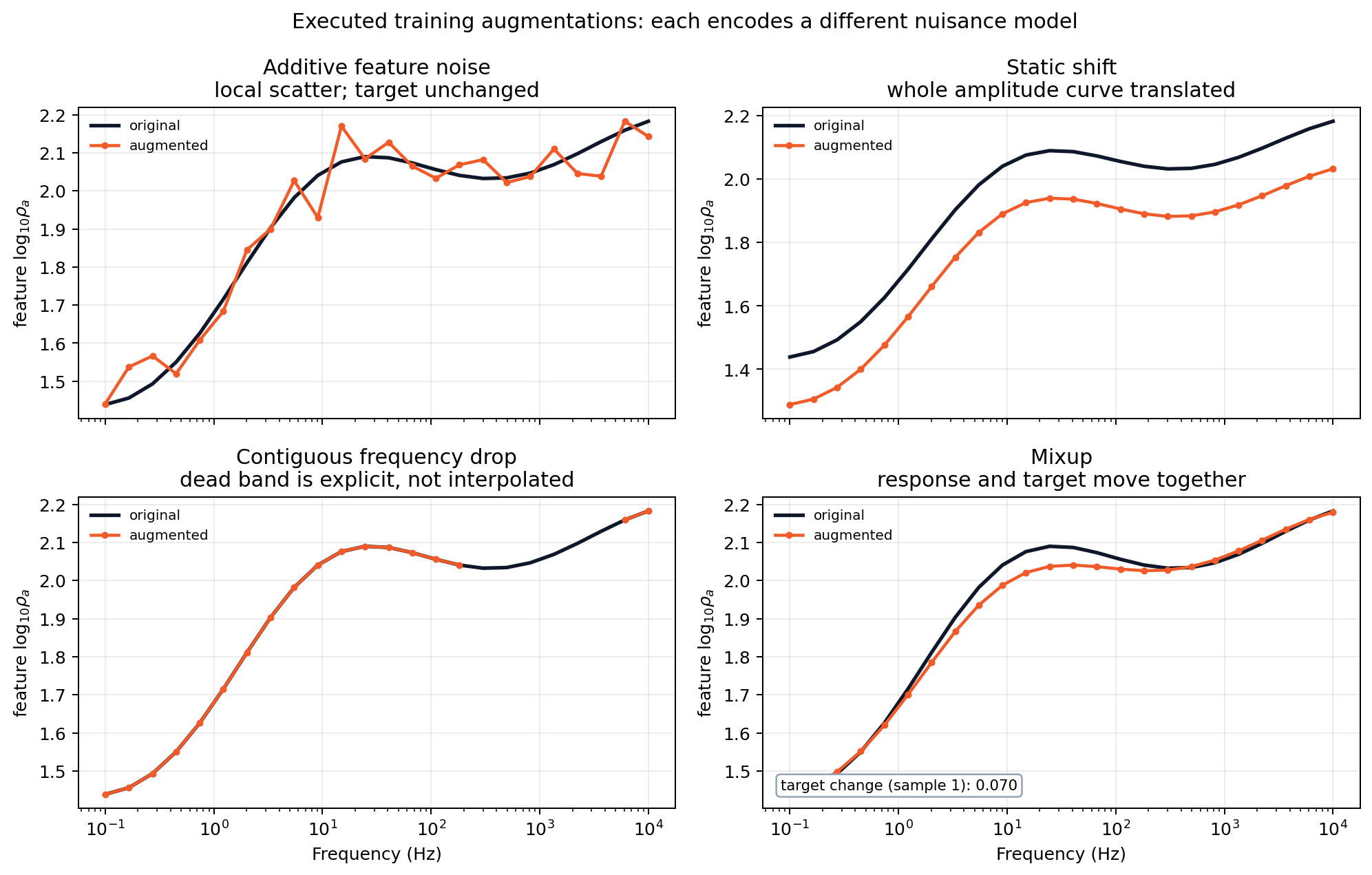
Four panels comparing an original response-like curve with noise, static-shift, contiguous-frequency-drop, and mixup augmentations executed by pyCSAMT — The public augmentation operators executed with fixed random generators. The panels show feature consequences rather than generic icons.#

Noise perturbs individual channels, whereas static shift translates the entire apparent-resistivity curve by one offset. The contiguous dropout panel preserves the location of a dead band instead of inventing measurements inside it. Mixup gives a smooth-looking curve, but its annotation confirms that the model target moved too; mixing only X would train against a false earth. Fit augmentation magnitudes from survey QC or a declared challenge model, and compare an unaugmented baseline through an ablation study.

The np.nan fill in this visual audit exists only to draw an obvious gap. Do not pass that array directly to a network: the current masked loss ignores non-finite targets, not non-finite inputs. For fitting, use a declared finite fill plus an explicit mask channel, or apply the same frozen imputation rule used at inference. Also note that AugmentNoise.phase_sigma is accepted by the current constructor but the implementation presently applies sigma to every feature. Until channel-specific noise is implemented and tested, split amplitude and phase arrays explicitly if they require different noise levels. Compose(seed=...) provides a shared repeatable random stream; record its seed separately from the train/validation split seed.

View and copy the executed augmentation auditClick to inspect and copy the complete code

def make_training_augmentation_audit() -> None:
    """Execute the public augmenters on response-like feature curves."""
    from pycsamt.ai.training import (
        AugmentFreqDrop,
        AugmentMixup,
        AugmentNoise,
        AugmentStaticShift,
    )

    frequency = np.logspace(-1, 4, 24)
    log_frequency = np.log10(frequency)
    x = np.stack(
        [
            1.8 + 0.32 * np.tanh(log_frequency - centre)
            + 0.08 * np.sin(1.8 * log_frequency + phase)
            for centre, phase in zip(np.linspace(0.4, 2.0, 8), np.linspace(0, 2, 8))
        ]
    ).astype(np.float32)
    y = np.stack([np.linspace(1.2 + 0.08 * i, 3.1 - 0.04 * i, 5)
                  for i in range(len(x))]).astype(np.float32)

    noisy, _ = AugmentNoise(sigma=0.06)(x, y, rng=np.random.default_rng(11))
    shifted, _ = AugmentStaticShift(
        shift_range=(0.5, 2.0), n_amp_features=24
    )(x, y, rng=np.random.default_rng(12))
    dropped, _ = AugmentFreqDrop(
        drop_rate=0.25, contiguous=True, fill_value=np.nan
    )(x, y, rng=np.random.default_rng(13))
    mixed, y_mixed = AugmentMixup(alpha=0.4)(
        x, y, rng=np.random.default_rng(14)
    )

    fig, axes = plt.subplots(2, 2, figsize=(11.2, 7.2), sharex=True)
    panels = [
        (noisy, "Additive feature noise", "local scatter; target unchanged"),
        (shifted, "Static shift", "whole amplitude curve translated"),
        (dropped, "Contiguous frequency drop", "dead band is explicit, not interpolated"),
        (mixed, "Mixup", "response and target move together"),
    ]
    for ax, (changed, title, subtitle) in zip(axes.flat, panels):
        ax.semilogx(frequency, x[0], color="#0f172a", lw=2.1, label="original")
        ax.semilogx(frequency, changed[0], color="#f15a29", lw=1.8,
                    marker="o", ms=3, label="augmented")
        ax.set(title=f"{title}\n{subtitle}", ylabel=r"feature $\log_{10}\rho_a$")
        ax.grid(alpha=0.22)
        ax.legend(frameon=False, fontsize=8)
    for ax in axes[-1]:
        ax.set_xlabel("Frequency (Hz)")
    axes[1, 1].text(
        0.03, 0.06,
        f"target change (sample 1): {np.linalg.norm(y_mixed[0] - y[0]):.3f}",
        transform=axes[1, 1].transAxes, fontsize=8.5,
        bbox={"boxstyle": "round,pad=0.3", "fc": "white", "ec": "#94a3b8"},
    )
    fig.suptitle("Executed training augmentations: each encodes a different nuisance model")
    fig.tight_layout()
    _save(fig, "training_augmentation_audit.png")

6.3.14.8. Monitor more than one loss#

The 1-D PyTorch trainer records training loss, validation loss, learning rate, and epoch time internally, and the checkpoint preserves training history and metadata. The internal _history attribute is useful for diagnostics but is private and therefore not a stable public API. Reporting code should tolerate its absence or consume history exposed by the agent workflow.

>>> history = {
...     "train_loss": [0.42, 0.31, 0.25, 0.23],
...     "val_loss": [0.45, 0.34, 0.33, 0.36],
...     "lr": [1e-3, 1e-3, 5e-4, 5e-4],
... }
>>> best = int(min(
...     range(len(history["val_loss"])),
...     key=history["val_loss"].__getitem__,
... ))
>>> print("best epoch:", best + 1)
best epoch: 3
>>> print("best validation loss:", history["val_loss"][best])
best validation loss: 0.33

For a fitted inverter, the same pattern is:

>>> history = getattr(inverter, "_history", None)
>>> if history:
...     best = int(min(
...         range(len(history["val_loss"])),
...         key=history["val_loss"].__getitem__,
...     ))
...     print("best epoch:", best + 1)
...     print("best validation loss:", history["val_loss"][best])

Interpret the curves jointly:

falling training and validation loss indicates useful learning;
falling training loss with rising validation loss indicates overfitting;
two flat, high curves suggest poor scaling, insufficient capacity, an unsuitable target representation, or weak information in the inputs;
erratic or non-finite loss calls for checks of learning rate, target range, invalid values, and gradient magnitude;
a low normalized loss can still hide large errors in a scientifically important layer, so inspect per-parameter errors in physical units.

The trainer is a validation-controlled state machine#

EMTrainer performs more than repeated gradient updates. It sends training batches through Adam, evaluates validation data without gradients or augmentation, passes validation loss to a learning-rate scheduler, increments the early stopping counter, and copies every genuinely improved state to CPU memory. After the loop, the copied best state replaces the last state. Consequently, the learning rate and the selected epoch are part of the result, not incidental console information.

The executed control audit below uses 360 training examples and 120 validation examples with four targets. Extra noise is deliberately added to the validation acquisition to create an irreducible floor; this is a controlled illustration of scheduler behavior, not a recommendation to corrupt validation data in a real experiment.

epochs completed: 120
restored best epoch: 108
best validation loss: 0.09802
initial / final learning rate: 0.003 / 0.0015
validation target RMSE: [0.320, 0.301, 0.280, 0.329]

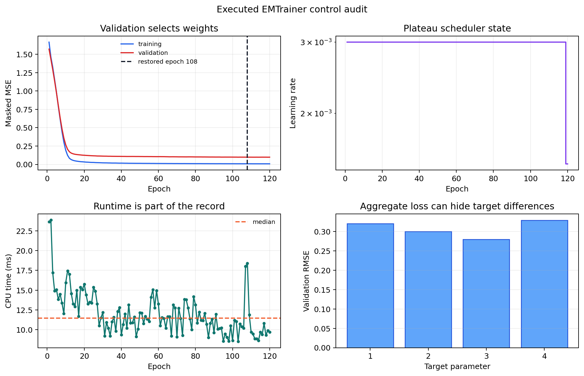
Executed EMTrainer audit showing training and validation losses, restored epoch, learning-rate reduction, CPU epoch timing, and per-target validation errors — One real `EMTrainer` run, including the validation decision variables that are often omitted from a loss plot.#

The validation curve reaches its useful floor while training loss continues to fall. The plateau scheduler halves the learning rate from \(3\times10^{-3}\) to \(1.5\times10^{-3}\), but the best state occurs at epoch 108 rather than at the final update. The timing panel also shows why runtime should be summarized by a median and spread rather than one unusually slow initialization epoch. Finally, the four target RMSE values differ even though optimization sees one scalar loss. For an earth model, replace those anonymous targets with layer resistivity, interface thickness, boundary depth, and response-space diagnostics in their physical units.

gradient clipping at norm 1.0 is active in this run. It limits an individual update; the history does not currently record how often clipping occurred, so a stable loss curve must not be interpreted as proof that the threshold was inactive. If clipping frequency matters to an experiment, instrument and archive it explicitly.

View and copy the executed trainer-control auditClick to inspect and copy the complete code

def make_training_trainer_controls() -> None:
    """Run EMTrainer and expose validation control, LR, timing, and recovery."""
    import torch
    from torch import nn
    from torch.utils.data import TensorDataset

    from pycsamt.ai.training import EMTrainer

    torch.manual_seed(29)
    rng = np.random.default_rng(29)
    x = rng.normal(size=(480, 12)).astype(np.float32)
    weights = rng.normal(scale=0.35, size=(12, 4)).astype(np.float32)
    y = (x @ weights + 0.18 * np.sin(x[:, :4])).astype(np.float32)
    y += rng.normal(scale=0.08, size=y.shape).astype(np.float32)
    # A noisier validation acquisition creates an honest irreducible floor,
    # making the scheduler and best-weight restoration visible in a short run.
    y[360:] += rng.normal(scale=0.30, size=y[360:].shape).astype(np.float32)
    train = TensorDataset(torch.from_numpy(x[:360]), torch.from_numpy(y[:360]))
    validation = TensorDataset(torch.from_numpy(x[360:]), torch.from_numpy(y[360:]))
    model = nn.Sequential(nn.Linear(12, 24), nn.ReLU(), nn.Linear(24, 4))
    trainer = EMTrainer(
        model, lr=3e-3, weight_decay=1e-5, patience=30,
        min_delta=1e-5, batch_size=48, device="cpu", grad_clip=1.0,
        verbose=False,
    ).fit(train, validation, epochs=120)
    history = trainer.history
    epoch = np.arange(1, len(history["train_loss"]) + 1)
    with torch.no_grad():
        predicted = trainer.model(torch.from_numpy(x[360:])).numpy()
    per_target_rmse = np.sqrt(np.mean((predicted - y[360:]) ** 2, axis=0))

    fig, axes = plt.subplots(2, 2, figsize=(10.8, 7.0))
    axes[0, 0].plot(epoch, history["train_loss"], color="#2563eb", label="training")
    axes[0, 0].plot(epoch, history["val_loss"], color="#dc2626", label="validation")
    axes[0, 0].axvline(trainer.best_epoch, color="#111827", ls="--",
                       label=f"restored epoch {trainer.best_epoch}")
    axes[0, 0].set(xlabel="Epoch", ylabel="Masked MSE", title="Validation selects weights")
    axes[0, 0].legend(frameon=False, fontsize=8)
    axes[0, 0].grid(alpha=0.22)
    axes[0, 1].step(epoch, history["lr"], where="post", color="#7c3aed")
    axes[0, 1].set(xlabel="Epoch", ylabel="Learning rate", title="Plateau scheduler state",
                   yscale="log")
    axes[0, 1].grid(alpha=0.22)
    axes[1, 0].plot(epoch, 1000 * np.asarray(history["epoch_time"]),
                    color="#0f766e", marker="o", ms=3)
    axes[1, 0].axhline(1000 * np.median(history["epoch_time"]), color="#f15a29",
                       ls="--", label="median")
    axes[1, 0].set(xlabel="Epoch", ylabel="CPU time (ms)", title="Runtime is part of the record")
    axes[1, 0].legend(frameon=False, fontsize=8)
    axes[1, 0].grid(alpha=0.22)
    axes[1, 1].bar(np.arange(1, 5), per_target_rmse, color="#60a5fa",
                   edgecolor="#1d4ed8")
    axes[1, 1].set(xlabel="Target parameter", ylabel="Validation RMSE",
                   title="Aggregate loss can hide target differences")
    axes[1, 1].set_xticks(np.arange(1, 5))
    axes[1, 1].grid(alpha=0.22, axis="y")
    fig.suptitle("Executed EMTrainer control audit")
    fig.tight_layout()
    _save(fig, "training_trainer_controls.png")
    print(
        "training controls:",
        {"epochs": len(epoch), "best_epoch": trainer.best_epoch,
         "best_val_loss": trainer.best_val_loss,
         "final_lr": history["lr"][-1],
         "target_rmse": per_target_rmse.tolist()},
    )

An executed CPU training audit#

The following small run is deliberately an execution and persistence test, not a production model. It keeps 15% of 240 synthetic examples completely outside fit, trains a compact FCN for at most 25 epochs, and reloads the checkpoint using the exact filename written by save.

>>> from pathlib import Path
>>> from tempfile import TemporaryDirectory
>>> import numpy as np
>>> from pycsamt.ai.inversion import EMInverter1D
>>> from pycsamt.forward.batch import generate_dataset

>>> frequency_hz = np.logspace(np.log10(1.01), 4, 24)
>>> samples = generate_dataset(
...     solver="mt1d", n_samples=240, freqs=frequency_hz,
...     n_layers=5, rho_range=(1.0, 10_000.0), depth_max=2000.0,
...     noise_level=0.05, noise_type="field", include_phase=True,
...     seed=137, n_jobs=1, output=None, verbose=False,
... )
>>> train, validation, external_test = samples.split(
...     val_frac=0.15, test_frac=0.15, seed=137
... )
>>> X_pool = np.vstack([train.X, validation.X])
>>> y_pool = np.vstack([train.y, validation.y])
>>> fitted = EMInverter1D(
...     n_features=48, n_layers=5, arch="fcn", solver="mt1d",
...     device="cpu", log_thickness=False, augment_noise=0.01,
... )
>>> _ = fitted.fit(
...     X_pool, y_pool, epochs=25, batch_size=64, lr=1e-3,
...     patience=7, val_frac=0.15, grad_clip=1.0, seed=137,
...     verbose=False,
... )
>>> predicted = fitted.predict(external_test.X)
>>> print("external test shape:", predicted.shape)
external test shape: (36, 9)
>>> print("stopped within budget:", len(fitted._history["train_loss"]) <= 25)
stopped within budget: True
>>> with TemporaryDirectory() as folder:
...     checkpoint = Path(folder) / "training_smoke.npz"
...     fitted.save(checkpoint)
...     restored = EMInverter1D.load(checkpoint)
...     restored_prediction = restored.predict(external_test.X)
...     print("checkpoint exists:", checkpoint.exists())
...     print("reload close:", np.allclose(
...         predicted, restored_prediction, rtol=1e-5, atol=1e-3
...     ))
checkpoint exists: True
reload close: True

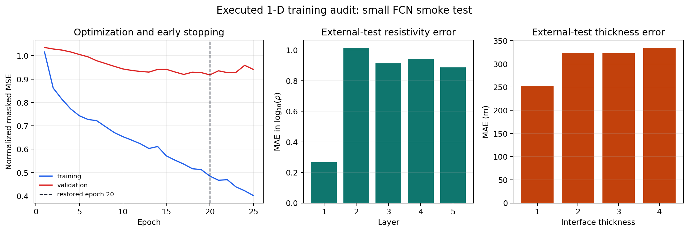
Executed FCN training convergence and physical-unit test errors — The validation minimum selects the restored epoch, whereas the right panel converts external-test errors back to target units. The run can converge in normalized space while deep interface-thickness errors remain hundreds of metres. This is why a checkpoint smoke test is necessary but insufficient for scientific acceptance.#

The widening train-validation gap and large held-out errors mean this small model should be rejected, even though fitting completed and restoration succeeded. Its value is to verify the mechanics and expose underpowered data and training choices before a costly production run.

The private _history access above is acceptable for this version-specific documentation audit, but production reporting should export a supported history artifact. The reload comparison uses a declared numerical tolerance; requiring bitwise equality across restored backends or hardware is generally too strict.

For reproducibility, the early-stopping rule can be written as a selection of the epoch

(4)#\[e^\star = \operatorname*{arg\,min}_{e\le E} \mathcal{L}_{\mathrm{val}}(e),\]

Equation (4) is subject to the patience rule. The final weights should be those from \(e^\star\), not necessarily the last epoch. Record both the last epoch and the selected epoch because a long tail of non-improving epochs can reveal optimizer instability or an overly patient run.

6.3.14.9. Training a 2-D U-Net#

EMInverter2D expects a batch of profile panels and matching resistivity images. Confirm the constructor dimensions and array axes against AI inversion data preparation before fitting.

>>> from pycsamt.ai.inversion import EMInverter2D
>>>
>>> inv2d = EMInverter2D(
...     n_components=4,
...     n_freqs=32,
...     n_stations=48,
...     n_depth=64,
...     solver="pytorch",
...     device="cpu",
... )
>>> print(inv2d.__class__.__name__, inv2d.n_components, inv2d.n_freqs, inv2d.n_stations, inv2d.n_depth)
EMInverter2D 4 32 48 64
>>> inv2d.fit(
...     X2_train_pool,
...     y2_train_pool,
...     epochs=200,
...     batch_size=16,
...     lr=1e-3,
...     patience=20,
...     val_frac=0.15,
...     grad_clip=1.0,
...     seed=42,
... )

The internal random split is along the profile-example axis, not the station axis inside a profile. Keep profiles descended from the same synthetic earth model in one external group. PyTorch and TensorFlow use different tensor layouts internally, and the TensorFlow path performs geometry resizing as needed; validate exported results on the requested depth and station grids. The current 2-D class does not expose the same documented public checkpoint workflow as EMInverter1D, so verify persistence requirements before a long production run.

The 2-D loss is an image-like objective, but the target is still a geophysical section. If \(U_{bzk}\) is log-resistivity for batch item \(b\), depth cell \(z\), and station \(k\), a masked section loss is

(5)#\[\mathcal{L}_{2D} = \frac{ \sum_{b,z,k} M_{bzk} \left(\hat{U}_{bzk}-U_{bzk}\right)^2 }{ \sum_{b,z,k} M_{bzk} }.\]

Pair equation (5) with boundary and response diagnostics. A visually smooth section can have low pixel loss while placing a conductor top at the wrong depth.

6.3.14.10. Training a graph model#

GCNInverter3D learns from station features and an adjacency matrix. Graph construction is part of the experiment, not a minor preprocessing detail.

>>> from pycsamt.ai.inversion import GCNInverter3D
>>>
>>> gcn = GCNInverter3D(
...     n_features=64,
...     n_layers=5,
...     solver="pytorch",
...     device="cpu",
... )
>>> print(gcn.__class__.__name__, gcn.n_features, gcn.n_layers)
GCNInverter3D 64 5
>>> gcn.fit(
...     X3_train_pool,
...     y3_train_pool,
...     adjacency=adjacency,
...     coords=station_xy,
...     epochs=250,
...     batch_size=8,
...     lr=1e-3,
...     patience=25,
...     val_frac=0.15,
...     seed=42,
... )

Audit node order, coordinate units, isolated nodes, degree distribution, and connected components. If neither a valid adjacency nor usable coordinates are supplied, an identity graph can be used as a fallback; that removes inter-station message passing and should never be mistaken for spatial inversion. Split along independent synthetic surveys. Do not split nodes from one survey between training and validation unless that transductive task is explicitly the scientific objective.

For graph training, write the graph construction rule beside the loss. If \(A\) is the adjacency matrix and \(H^{(t)}\) is a hidden node matrix, the GCN update is conditioned on a neighborhood aggregation of the form

(6)#\[H^{(t+1)} = \sigma\!\left(\tilde{A}H^{(t)}W^{(t)}\right),\]

In equation (6), \(\tilde{A}\) is the normalized adjacency used by the implementation. Changing coordinate units, edge radius, or node order changes \(\tilde{A}\) and therefore changes the model being trained.

6.3.14.11. Joint and ensemble training#

A JointInverter receives one feature matrix per modality. All matrices and the target must share the same row order.

>>> from pycsamt.ai.inversion import JointInverter
>>>
>>> joint = JointInverter(
...     n_features_list=(64, 25),
...     n_layers=5,
...     solver="pytorch",
... )
>>> print(joint.__class__.__name__, joint.n_features_list, joint.n_layers)
JointInverter (64, 25) 5
>>> joint.fit(
...     [X_mt_train_pool, X_aux_train_pool],
...     y_train_pool,
...     epochs=250,
...     batch_size=128,
...     lr=1e-3,
...     patience=25,
...     val_frac=0.15,
...     seed=42,
... )

Test a shuffled or missing auxiliary modality as an ablation. If performance does not change, the claimed joint information may not be used. Remember that the current joint trainer also estimates its modality normalizers before its internal split.

Joint training is vulnerable to row-alignment errors because all modalities share a target. A safe pre-fit invariant is

(7)#\[\operatorname{id}^{(1)}_i = \operatorname{id}^{(2)}_i = \operatorname{id}^{(y)}_i \quad \text{for every row } i.\]

Equation (7) must be checked explicitly. Do not rely on array length alone. Equal lengths can still describe different stations, times, or synthetic parent models if the join order was lost.

EnsembleInverter deep-copies and trains the base estimator with different seeds:

>>> from pycsamt.ai.inversion import EMInverter1D, EnsembleInverter
>>>
>>> base = EMInverter1D(
...     n_features=64,
...     n_layers=5,
...     solver="mt1d",
... )
>>> ensemble = EnsembleInverter(base, n_estimators=5, seeds=[42, 43, 44, 45, 46])
>>> print(ensemble.__class__.__name__, ensemble.n_estimators, ensemble.seeds[:2])
EnsembleInverter 5 [42, 43]
>>> ensemble.fit(
...     X_train_pool,
...     y_train_pool,
...     epochs=250,
...     batch_size=256,
...     patience=25,
...     val_frac=0.15,
...     verbose=True,
... )
>>> ensemble.save("checkpoints/mt1d_ensemble")

Budget approximately one full training run per member. Member seeds affect both the random split and model optimization, so ensemble spread combines those sources of variation. In uncertainty language, ensembles mainly probe epistemic uncertainty; input noise and incomplete measurements contribute aleatoric uncertainty. Calibrate prediction intervals only on a separate calibration set. Persist calibration products separately because the current ensemble checkpoint does not preserve fitted calibrators.

6.3.14.12. PINN and hybrid optimization#

Do not transfer the supervised recipe mechanically to a PINN or hybrid run. Both workflows must track the data-misfit term, physics residual, regularization terms, their weights, forward-solver settings, and the initial model. A low total loss is ambiguous if one weighted term dominates. See Hybrid AI and physics inversion and Physics-informed 2-D inversion for the staged workflow and required diagnostics.

6.3.14.13. Reproducible experiment design#

One successful seed is not a stability study. For model comparison:

freeze one external test set and one grouping policy;
train each candidate with several declared seeds;
select hyperparameters using validation results only;
report the distribution of physical-unit metrics across seeds;
compare forward-response misfit and geological plausibility;
retain the configuration, dataset identity, logs, environment, and model artifact for every accepted run.

Changing the seed changes both the high-level internal validation membership and weight initialization. If the experiment must isolate initialization variance from split variance, construct a lower-level training protocol with a frozen split rather than interpreting the high-level seed sweep as a pure initialization test.

6.3.14.14. Failure diagnosis#

Non-finite loss: Check input and target finiteness, logarithms of non-positive values, extreme parameter bounds, learning rate, and gradient norms. Do not simply discard the failing batches.
Validation loss rises early: Confirm grouping, reduce capacity, increase representative training data, review augmentation, and shorten patience. First rule out duplicated parent models across splits.
Training and validation losses remain high: Verify component order and units, input/target pairing, layer layout, and whether the response contains enough information for the requested model.
Good synthetic metrics but poor field behavior: Suspect domain shift: acquisition geometry, frequency coverage, noise, distortion, geology, or preprocessing differs from the simulator. More epochs usually amplify rather than solve this problem.
Unstable graph training: Inspect node ordering, coordinate scale, adjacency normalization, disconnected components, and survey-level splits.
Out-of-memory errors: Reduce batch size first, then model width or panel dimensions. Record the changed setting because it can alter optimizer behavior.

6.3.14.15. Training completion checklist#

Before promoting a model to inference, confirm that:

the external test set was never passed to fit;
dataset identity, split policy, seeds, versions, and device were recorded;
the selected epoch came from validation behavior, not test performance;
losses and physical-unit errors were checked per parameter or depth range;
predicted models were forward-modelled and compared with held-out responses;
noise, domain-shift, and out-of-distribution tests were run;
checkpoint loading and one representative prediction were verified;
known normalization and persistence limitations were written into the run report rather than hidden.

Training is complete only when the artifact and the evidence needed to reject or trust it are both reproducible. Continue with AI inversion inference, AI inversion uncertainty, and AI inversion reporting.

The executed audit figures are reproduced by docs/scripts/generate_ai_inversion_figures.py using deterministic synthetic generation and a CPU PyTorch run. Small numerical differences may occur across backend and library versions; the scientific conclusion depends on the loss separation and physical-unit errors, not identical pixels or last decimals.