Phase-tensor dimensionality: rule-based and dictionary-learned (pycsamt.emtools.dimensionality)

pycsamt.emtools.dimensionality classifies each (station, frequency) as 1-D, 2-D, or 3-D from the phase tensor’s Bibby (2005) skew angle \(\beta\) and ellipticity, then offers a second, independent route to the same question: standardize four impedance/phase-tensor features and learn a small sparse dictionary (MOD + ISTA) over them, producing an unsupervised, data-driven dimensionality label to compare against the rule-based one. On top of both routes sit masking helpers (drop frequencies judged too 3-D) and a strike-rotation + antisymmetrization step meant to prepare data for 2-D inversion.

This example uses L18PLT (data/AMT/WILLY_DATA/), the same CSAMT-band line used in the anisotropy/csumt/diag examples.

Warning

Building this example surfaced four real, independent bugs in dimensionality.py, all now fixed:

1. plot_dim_map() looked up coordinates via ed.lat/.latitude/.lon/.longitude, attributes the real Site class does not have (it exposes a single .coords property returning (lat, lon, elev)) — so it always fell through to “no coords”, even for this line, which does have real, valid coordinates.

2. project_to_2d()’s strike=None (auto-strike) path called pycsamt.site.edit.rotate_to_strike, which does not exist (rotate_to_strike lives in pycsamt.emtools.tensor, not pycsamt.site.edit) — an AttributeError every time.

3. Its explicit strike=<value> path called pycsamt.site.edit.rotate(S, angle=..., inplace=...), but that function’s parameter is named angle_deg, not angle — a TypeError every time. Both paths were completely broken; pycsamt.emtools.tensor already has correctly working rotate / rotate_to_strike wrappers, now reused instead.

4. learn_dim_dictionary()’s training loop computed the dictionary update, then transposed it again before reassigning it (D = _mod_update(Z.T, A).T) — _mod_update already returns the correctly-oriented matrix, so this flipped its shape and crashed every run with the default n_iter=40 on the second iteration. No test in the repository exercised any of these four paths.

1. Raw features for one station

phase_features_table() derives four per-(station, frequency) features from the phase tensor and impedance: Bibby skew \(|\beta|\), ellipticity, log10(ρ_det), and the determinant phase. Plotting the two features the rule-based classifier actually uses, against its own default thresholds, shows exactly what the classifier sees before any labelling happens.

import matplotlib.pyplot as plt
import numpy as np
import pandas as pd
from _datasets import load_survey

from pycsamt.emtools import (
    classify_dimensionality,
    encode_dimensionality,
    learn_dim_dictionary,
    mask_by_dictionary,
    mask_by_dimensionality,
    phase_features_table,
    plot_atom_psection,
    plot_dim_confidence_grid,
    plot_dim_map,
    plot_dim_occupancy_area,
    project_to_2d,
)

SKEW_TH, ELLIPT_TH = 3.0, 0.2  # module defaults

survey = load_survey("amt_l18plt")
features = phase_features_table(survey)
station = "18-001A"
d = features[features["station"] == station].sort_values("period")

fig, (ax1, ax2) = plt.subplots(2, 1, figsize=(7, 6), sharex=True)
ax1.semilogx(d["period"], d["beta_abs"], "o-", ms=3, color="#1f77b4")
ax1.axhline(SKEW_TH, color="0.3", ls="--", lw=1, label=f"skew_th={SKEW_TH:g}")
ax1.set_ylabel(r"$|\beta|$ (deg)")
ax1.legend(fontsize=8)
ax1.set_title(f"{station} — dimensionality features vs. period")

ax2.semilogx(d["period"], d["ellipt_abs"], "o-", ms=3, color="#d62728")
ax2.axhline(
    ELLIPT_TH, color="0.3", ls="--", lw=1, label=f"ellipt_th={ELLIPT_TH:g}"
)
ax2.set_ylabel("ellipticity")
ax2.set_xlabel("Period (s)")
ax2.legend(fontsize=8)
fig.tight_layout()

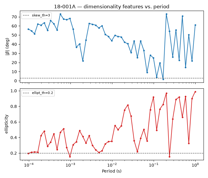
Reading this figure. \(|\beta|\) for this station sits at 20-60°, roughly an order of magnitude above the 3° default threshold, across almost the entire recorded band; ellipticity is likewise mostly well above 0.2. On the classifier’s own rule (both must be at or below their threshold to qualify as 1-D/2-D), essentially every frequency at this station reads as 3-D — worth keeping in mind before the survey-wide view below.

2. How the rule partitions feature space

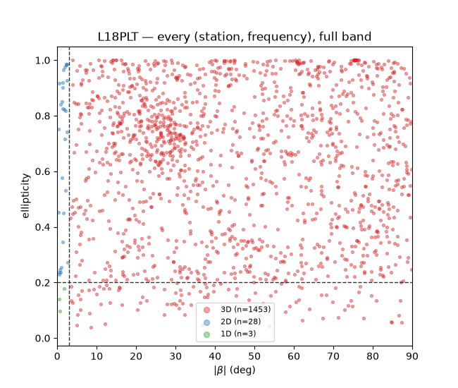
classify_dimensionality() labels every (station, frequency) 0 (1-D), 1 (2-D), or 2 (3-D) from exactly the two features above. Plotting every point in that 2-D feature space at once, with the threshold lines drawn in, makes the rule’s geometry — and how much of the real data falls outside it — directly visible.

dim_df = classify_dimensionality(survey)
colors = {0: "#2ca02c", 1: "#1f77b4", 2: "#d62728"}
labels = {0: "1D", 1: "2D", 2: "3D"}

fig, ax = plt.subplots(figsize=(6.5, 5.5))
for k in (2, 1, 0):  # draw 3D first so 1D/2D aren't hidden underneath
    m = dim_df["dim"] == k
    ax.scatter(
        dim_df.loc[m, "beta_abs"],
        dim_df.loc[m, "ellipt_abs"],
        s=8,
        alpha=0.4,
        color=colors[k],
        label=f"{labels[k]} (n={int(m.sum())})",
    )
ax.axvline(SKEW_TH, color="0.2", ls="--", lw=1)
ax.axhline(ELLIPT_TH, color="0.2", ls="--", lw=1)
ax.set_xlabel(r"$|\beta|$ (deg)")
ax.set_ylabel("ellipticity")
ax.set_xlim(0, 90)
ax.legend(fontsize=8, markerscale=2)
ax.set_title("L18PLT — every (station, frequency), full band")

Text(0.5, 1.0, 'L18PLT — every (station, frequency), full band')

Reading this figure. The 1-D/2-D region — left of the vertical and, for 2-D, above the horizontal line — holds only a thin sliver of points (3/1484 1-D, 28/1484 2-D); the rest of the whole survey sits in the 3-D region to the right. This is not one noisy station; it is the entire line at the classifier’s default thresholds.

3. How sensitive is that to the threshold?

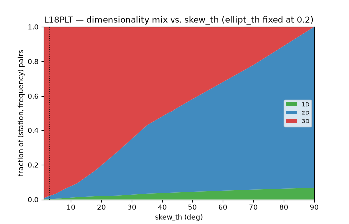
Since almost everything reads “3-D” at the default 3° skew threshold, a natural question is how much of that is a genuinely severe response versus a threshold picked for cleaner (e.g. regional MT) data. Sweeping skew_th while holding ellipt_th fixed answers it directly.

b = dim_df["beta_abs"].to_numpy()
e = dim_df["ellipt_abs"].to_numpy()
skew_ths = np.array([1, 2, 3, 5, 8, 12, 18, 25, 35, 50, 70, 90], dtype=float)
frac_1d, frac_2d, frac_3d = [], [], []
for sth in skew_ths:
    ok2 = b <= sth
    d0 = (ok2 & (e <= ELLIPT_TH)).mean()
    d1 = (ok2 & (e > ELLIPT_TH)).mean()
    frac_1d.append(d0)
    frac_2d.append(d1)
    frac_3d.append(1.0 - d0 - d1)

fig, ax = plt.subplots(figsize=(7, 4.5))
ax.stackplot(
    skew_ths,
    frac_1d,
    frac_2d,
    frac_3d,
    colors=[colors[0], colors[1], colors[2]],
    labels=["1D", "2D", "3D"],
    alpha=0.85,
)
ax.axvline(SKEW_TH, color="black", ls=":", lw=1.2)
ax.set_xlabel("skew_th (deg)")
ax.set_ylabel("fraction of (station, frequency) pairs")
ax.set_xlim(skew_ths.min(), skew_ths.max())
ax.set_ylim(0, 1)
ax.legend(fontsize=8, loc="center right")
ax.set_title(
    "L18PLT — dimensionality mix vs. skew_th (ellipt_th fixed at 0.2)"
)

Text(0.5, 1.0, 'L18PLT — dimensionality mix vs. skew_th (ellipt_th fixed at 0.2)')

Reading this figure. The 3-D fraction falls smoothly and monotonically from 99.3% at skew_th=1° to 0% only at skew_th=90° — the mathematical ceiling of \(|\beta|\) itself, not a realistic setting. Even a generously relaxed skew_th=25° — nearly 10x the textbook default — still classifies 73% of this survey as 3-D. There is no threshold in a realistic range that makes this line look predominantly 1-D/2-D; that is a property of the data, not a knob to tune away.

4. The module’s pseudo-section and occupancy views

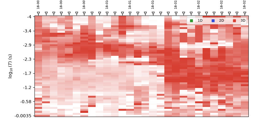
plot_dim_confidence_grid() maps the same labels onto a station x period grid, with a classification confidence margin driving the opacity.

plot_dim_confidence_grid(survey)

<Axes: xlabel='Station', ylabel='$\\log_{10}(T)$ (s)'>

Reading this figure. The grid is almost solid red (3-D) with visibly varying opacity (confidence) cell to cell, and no blue/green (2-D/1-D) survives being visible at this resolution — consistent with only 31 of 1484 station-frequency pairs qualifying as 1-D/2-D at all (section 2), too sparse to show up as more than the occasional lighter red cell here.

plot_dim_occupancy_area(survey)

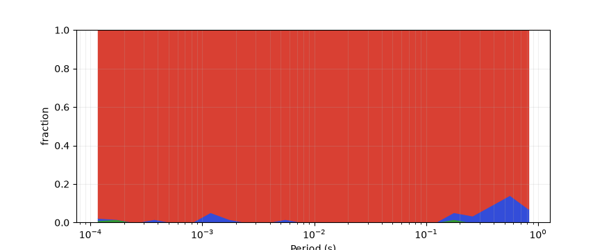
<Axes: xlabel='Period (s)', ylabel='fraction'>

Reading this figure. plot_dim_occupancy_area() collapses the grid to a per-period-band stacked fraction — the same “almost entirely 3-D” result from section 2 and 3, but now split out across the recorded period band rather than pooled into one number, confirming it holds at essentially every period, not just on average.

5. Mapping dimensionality in space

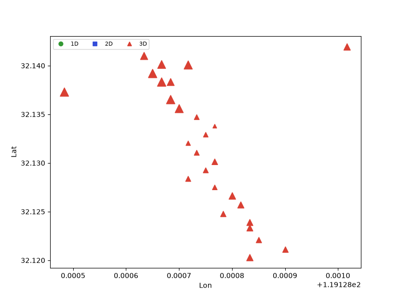
plot_dim_map() needed the .coords fix above to work at all; with it, station markers are coloured/shaped by class and sized by confidence at one target period.

plot_dim_map(survey, period=0.01)

<Axes: xlabel='Lon', ylabel='Lat'>

Reading this figure. At T = 0.01 s, all 28 stations come back as red triangles (3-D) — the map view of the same result, station by station, rather than averaged over the whole line.

6. Advanced: does 2-D projection actually help?

project_to_2d() rotates to a best-fit strike and antisymmetrizes the off-diagonal tensor — a standard step before 2-D inversion. Whether it meaningfully reduces the classified 3-D fraction, rather than just being assumed to help, is worth checking rather than asserting.

projected = project_to_2d(survey, method="swift")
dim_after = classify_dimensionality(projected)

before_frac = (
    dim_df["dim"].value_counts(normalize=True).reindex([0, 1, 2]).fillna(0.0)
)
after_frac = (
    dim_after["dim"]
    .value_counts(normalize=True)
    .reindex([0, 1, 2])
    .fillna(0.0)
)

fig, ax = plt.subplots(figsize=(6, 4.5))
x = np.arange(3)
w = 0.35
ax.bar(
    x - w / 2, before_frac.to_numpy(), width=w, label="before", color="0.6"
)
ax.bar(
    x + w / 2,
    after_frac.to_numpy(),
    width=w,
    label="after project_to_2d",
    color="#d62728",
)
ax.set_xticks(x, ["1D", "2D", "3D"])
ax.set_ylabel("fraction")
ax.legend(fontsize=8)
ax.set_title("Effect of strike rotation + antisymmetrization")

print(
    f"mean |beta|: before={dim_df['beta_abs'].mean():.1f} deg, "
    f"after={dim_after['beta_abs'].mean():.1f} deg"
)
print(
    f"mean ellipticity: before={dim_df['ellipt_abs'].mean():.3f}, "
    f"after={dim_after['ellipt_abs'].mean():.3f}"
)

/opt/build/repo/pycsamt/z/utils.py:396: ComplexWarning: Casting complex values to real discards the imaginary part
  E = ensure_z3(z_err).astype(float, copy=False)
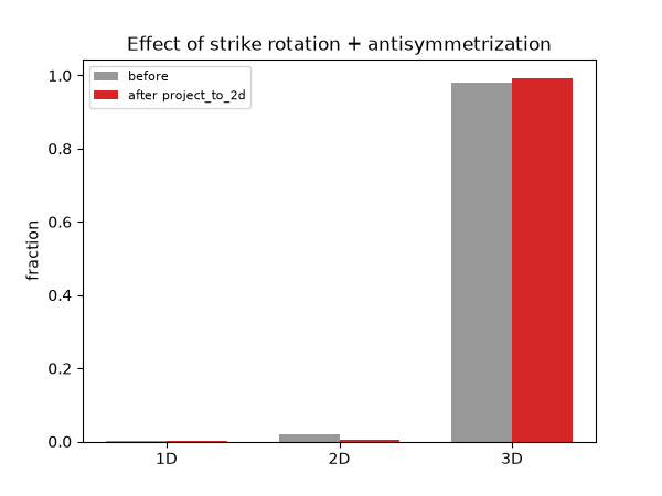
mean |beta|: before=44.5 deg, after=44.3 deg
mean ellipticity: before=0.625, after=0.407

Reading this figure. Mean \(|\beta|\) and mean ellipticity both drop slightly after projection (about 44.5°→41.5° and 0.63→0.51), yet the classified 3-D fraction does not improve — it edges up slightly (97.9%→99.6%), because mean \(|\beta|\) is still an order of magnitude above the 3° threshold, so a small average improvement moves almost no points across the boundary while a few marginal 2-D cases tip the other way. Antisymmetrization/strike rotation is a real, useful regularization step for 2-D inversion, but it is not a fix for data that is this far from 1-D/2-D by the classifier’s own rule — don’t expect it to change a “mostly 3-D” verdict into a “mostly 2-D” one.

7. Advanced: an unsupervised second opinion

learn_dim_dictionary() learns a small sparse dictionary over the four standardized features (MOD + ISTA), with no thresholds at all; each station-frequency is then re-encoded and labelled by its dominant atom via encode_dimensionality().

model = learn_dim_dictionary(survey, n_atoms=6, n_iter=40, code_iter=50)
encoded = encode_dimensionality(survey, model)

agree = (dim_df["dim"].to_numpy() == encoded["dim_pred"].to_numpy()).mean()
print(f"rule vs. dictionary agreement: {agree:.1%}")
print("rule-based:", dim_df["dim"].value_counts().to_dict())
print("dictionary:", encoded["dim_pred"].value_counts().to_dict())

fig, ax = plt.subplots(figsize=(5.5, 5))
confusion = pd.crosstab(
    dim_df["dim"].map(labels), encoded["dim_pred"].map(labels)
)
confusion = confusion.reindex(
    index=["1D", "2D", "3D"], columns=["1D", "2D", "3D"], fill_value=0
)
im = ax.imshow(confusion.to_numpy(), cmap="Blues")
ax.set_xticks(range(3), confusion.columns)
ax.set_yticks(range(3), confusion.index)
ax.set_xlabel("dictionary label")
ax.set_ylabel("rule-based label")
for i in range(3):
    for j in range(3):
        v = confusion.to_numpy()[i, j]
        ax.text(
            j,
            i,
            str(v),
            ha="center",
            va="center",
            color="white" if v > confusion.to_numpy().max() / 2 else "black",
        )
ax.set_title(f"Rule vs. dictionary — {agree:.0%} agreement")
fig.colorbar(im, ax=ax, shrink=0.8, label="count")

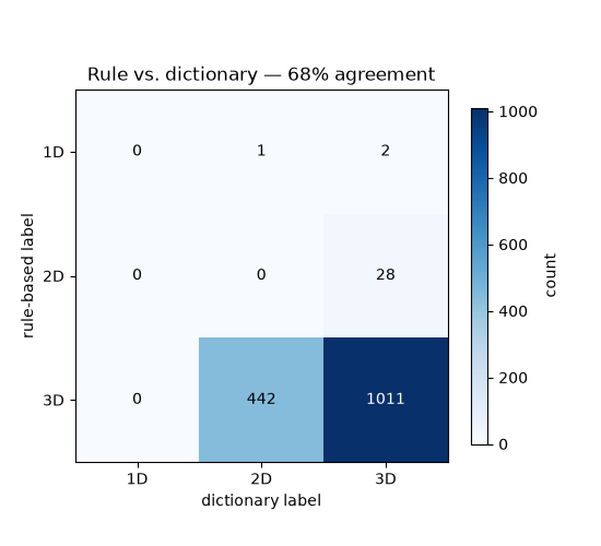
rule vs. dictionary agreement: 68.1%
rule-based: {2: 1453, 1: 28, 0: 3}
dictionary: {2: 1041, 1: 443}

<matplotlib.colorbar.Colorbar object at 0x7f2aa48e3470>

Reading this figure. The two independent methods agree on about 68% of all 1484 station-frequency pairs — meaningful agreement, but nowhere near total. The learned dictionary never assigns a 1-D label at all (no atom’s mean feature values fall under the rule’s 1-D corner), and it calls a substantial fraction of the rule-based 3-D population “2-D” instead. That is a genuine, useful disagreement to know about: the two methods encode different notions of “how far from 1-D”, and neither should be taken as unquestionably correct on its own — cross-checking one against the other, as done here, is exactly the point of having both in the same module.

plot_atom_psection(survey, model)

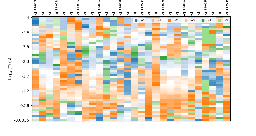
<Axes: xlabel='Station', ylabel='$\\log_{10}(T)$ (s)'>

Reading this figure. plot_atom_psection() shows which learned atom dominates at each station and period, with opacity set by that atom’s coding energy — the dictionary-learning counterpart to the rule-based pseudo-section in section 4, at the level of individual learned components rather than a single 1D/2D/3D label.

8. Masking: how much of the survey would either method keep?

Both mask_by_dimensionality() and mask_by_dictionary() NaN-out frequencies judged too 3-D, ready for an inversion step that tolerates missing frequencies. Setting NaN into a tensor logs an internal “Z must be finite” notice per site from the Z-object’s own setter — expected here, not a new problem — so logging is quieted for this step.

import logging  # noqa: E402

logging.disable(logging.ERROR)
try:
    masked_rule = mask_by_dimensionality(survey, keep=(0, 1))
    masked_dict = mask_by_dictionary(survey, model, keep=(0, 1))
finally:
    logging.disable(logging.NOTSET)


def _frac_masked(sites) -> float:
    from pycsamt.emtools._core import (
        _get_z_block,
        _iter_items,
    )

    n_tot = n_nan = 0
    for ed in _iter_items(sites):
        _, z, fr = _get_z_block(ed)
        if z is None:
            continue
        n_tot += fr.size
        n_nan += int(np.isnan(z[:, 0, 1]).sum())
    return n_nan / n_tot if n_tot else float("nan")


print(
    f"rule-based mask (keep 1D+2D) discards {_frac_masked(masked_rule):.1%} of the survey"
)
print(
    f"dictionary mask (keep 1D+2D) discards {_frac_masked(masked_dict):.1%} of the survey"
)

rule-based mask (keep 1D+2D) discards 97.9% of the survey
dictionary mask (keep 1D+2D) discards 70.1% of the survey

Reading this output. Keeping only what the rule calls 1-D/2-D throws away 97.9% of this line — in practice unusable without relaxing skew_th/ellipt_th well beyond their defaults first (section 3 shows what that costs). The dictionary-based mask is markedly less aggressive, discarding about 70% — consistent with it calling more of the survey “2-D” in the confusion matrix above. Which one is “right” depends on how conservative the downstream 2-D inversion needs to be; this module gives you both answers rather than picking one silently.