Frequency Editing, Resampling, And QC

pycsamt.emtools.frequency is the user-guide hub for operations that change, evaluate, or visualize the frequency axis. It is used before inversion, before section plotting, after quality control, and whenever multiple stations need to share a consistent frequency grid.

The module covers four practical jobs:

• selecting a usable frequency band;

• dropping, masking, or recovering low-confidence rows;

• regridding, decimating, smoothing, and aligning station grids;

• plotting frequency coverage, apparent depth, and band-level summary diagnostics.

Full callable signatures live in the API reference. This page focuses on how to use the workflows safely, how to read their tables, and how to avoid common frequency-axis traps.

Why Frequency Editing Matters

CSAMT/AMT/MT processing is rarely limited by one bad station value. More often, a workflow succeeds or fails because the frequency axis is inconsistent, too noisy at the band edges, or incompatible across stations. A 2-D inversion, pseudo-section, or model-comparison workflow needs clear decisions about:

• which band is physically meaningful;

• which frequency rows are trusted;

• whether bad rows are removed or kept as missing values;

• whether stations should be interpolated to a shared grid;

• whether smoothing or decimation is acceptable for the next step.

The frequency module makes those decisions explicit and auditable.

Data Contract

All editing functions accept the usual emtools input:

• a directory containing EDI files,

• one EDI-like object,

• a Sites container,

• an iterable of site-like objects.

Internally the functions call ensure_sites. The familiar recursive, on_dup, strict, and verbose arguments behave the same way as in the rest of the user guide.

Most editing functions default to inplace=False. Keep that default while exploring. Switch to inplace=True only when you intentionally want to mutate the input object.

Selecting A Band

Use select_band when you already know the frequency limits.

from pathlib import Path

from pycsamt.emtools.frequency import select_band

edi_dir = Path("data/AMT/WILLY_DATA/L18PLT")

mid_band = select_band(
    edi_dir,
    fmin=10.0,
    fmax=1000.0,
    inplace=False,
)

fmin and fmax are in hertz. The convenience argument band_hz=(10.0, 1000.0) is also accepted. If both forms are provided, explicit fmin and fmax take precedence.

Use keep when you want specific frequencies rather than a continuous band.

from pycsamt.emtools.frequency import select_band

selected = select_band(
    "data/AMT/WILLY_DATA/L18PLT",
    keep=[10.0, 100.0, 1000.0],
)

Band selection removes rows outside the chosen band. It changes the frequency grid length.

Removing Duplicate Frequencies

Use drop_duplicates when a station has repeated or unsorted frequency rows.

from pycsamt.emtools.frequency import drop_duplicates

cleaned = drop_duplicates(
    "data/AMT/WILLY_DATA/L18PLT",
    tol=1e-10,
    inplace=False,
)

The function keeps the first occurrence of each frequency within the tolerance and applies the same row selection to impedance and tipper blocks when present.

Frequency Confidence

Confidence-based editing uses frequency_confidence_table from the QC workflow. The frequency module computes that table internally, but you should inspect it before editing.

import matplotlib.pyplot as plt

from pycsamt.emtools.qc import frequency_confidence_table

survey = "data/AMT/WILLY_DATA/L18PLT"
confidence = frequency_confidence_table(survey)

print(confidence[["station", "frequency_hz", "confidence", "flags"]].head())
print(confidence["confidence"].describe())

station = "18-001A"
one = confidence.loc[confidence["station"] == station].sort_values("period_s")

fig, ax = plt.subplots(figsize=(7, 4.5))
ax.semilogx(one["period_s"], one["confidence"], "o-")
ax.axhline(0.90, color="tab:red", linestyle="--", label="ci_hi")
ax.axhline(0.50, color="tab:orange", linestyle="--", label="ci_lo")
ax.set_xlabel("Period (s)")
ax.set_ylabel("Confidence")
ax.legend()
fig.tight_layout()

   station  ...                                              flags
0  18-001A  ...  recoverable,high_error,offdiag_mismatch,diagon...
1  18-001A  ...  reject,high_error,offdiag_mismatch,diagonal_le...
2  18-001A  ...  reject,high_error,offdiag_mismatch,diagonal_le...
3  18-001A  ...  reject,high_error,offdiag_mismatch,diagonal_le...
4  18-001A  ...  reject,high_error,offdiag_mismatch,diagonal_le...

[5 rows x 4 columns]
count    1484.000000
mean        0.658116
std         0.096143
min         0.417464
25%         0.586675
50%         0.654938
75%         0.736039
max         0.863041
Name: confidence, dtype: float64

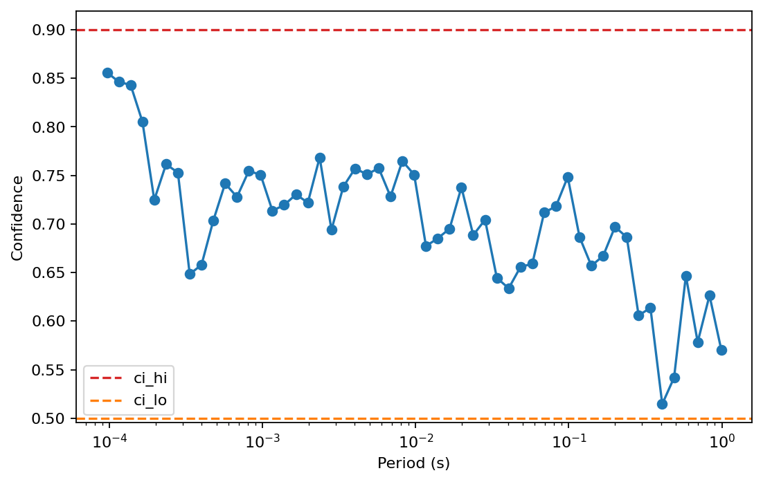
The key lesson is simple: do not choose ci_hi or threshold before looking at the confidence distribution. If no row reaches ci_hi, recovery has no trusted rows to interpolate from.

Drop Or Mask Low-Confidence Rows

Dropping removes rows from the frequency grid. Masking keeps the grid but replaces low-confidence tensor rows with NaN.

from pycsamt.emtools.frequency import (
    drop_low_confidence_frequencies,
    mask_low_confidence_frequencies,
)

survey = "data/AMT/WILLY_DATA/L18PLT"

dropped = drop_low_confidence_frequencies(
    survey,
    threshold=0.50,
    also="both",
    inplace=False,
)

masked = mask_low_confidence_frequencies(
    survey,
    threshold=0.50,
    also="both",
    inplace=False,
)

Use drop when downstream code cannot handle missing rows. Use mask when preserving the original frequency grid matters, for example when comparing before and after processing.

The also argument controls which blocks are edited:

Value	Meaning
"z"	Edit impedance only.
"tipper"	Edit tipper only.
"both"	Edit impedance and tipper when present.

Recover Low-Confidence Rows

recover_low_confidence_frequencies treats rows in [ci_lo, ci_hi) as recoverable and interpolates them from trusted rows whose confidence is at least ci_hi. Rows below ci_lo are handled by reject.

from pycsamt.emtools.frequency import recover_low_confidence_frequencies

recovered = recover_low_confidence_frequencies(
    "data/AMT/WILLY_DATA/L18PLT",
    ci_hi=0.72,
    ci_lo=0.50,
    interpolation="linear",
    reject="drop",
    also="both",
    inplace=False,
)

Valid interpolation modes are "linear" and "nearest". Valid reject modes are:

Reject mode	Meaning
"drop"	Remove rows below ci_lo.
"mask"	Keep rows below ci_lo but set them to NaN.
"keep"	Leave rejected rows unchanged.

Recovery is interpolation, not magic. At band edges, interpolation can behave like holding the nearest trusted value. Always inspect the result when many rows are recovered.

High-Level Editing Workflow

Use edit_frequencies_by_confidence when you want the edited sites, a station-level report, and a row-level decision table in one object.

from pycsamt.emtools.frequency import edit_frequencies_by_confidence

result = edit_frequencies_by_confidence(
    "data/AMT/WILLY_DATA/L18PLT",
    mode="recover",
    ci_hi=0.72,
    ci_lo=0.50,
    reject="drop",
    interpolation="linear",
    api=False,
)

print(result.summary())
print(result.report.head())
print(result.decisions.head())

FrequencyEditResult(mode='recover', method='composite', dropped=73, masked=102, recovered=867)
   station  n_freq_before  ...  n_masked_or_unfinite  confidence_delta
0  18-001A             53  ...                     0          0.027413
1  18-002U             53  ...                     0         -0.038885
2  18-003A             53  ...                     3          0.061644
3  18-004A             53  ...                     3         -0.026442
4  18-005U             53  ...                     1          0.026781

[5 rows x 18 columns]
   station  frequency_hz  period_s  ...  present_after  finite_after action
0  18-001A       10400.0  0.000096  ...           True          True   kept
1  18-001A        8707.0  0.000115  ...           True          True   kept
2  18-001A        7289.0  0.000137  ...           True          True   kept
3  18-001A        6102.0  0.000164  ...           True          True   kept
4  18-001A        5108.0  0.000196  ...           True          True   kept

[5 rows x 10 columns]

result is a FrequencyEditResult with:

• sites: edited sites.

• report: station-level before/after table.

• decisions: one row per original station-frequency row.

• n_dropped, n_masked, n_recovered: convenience counts.

• mode, method, ci_hi, ci_lo, reject, interpolation: edit metadata.

For in-memory objects, pass an independent before_sites when you need an untouched baseline for reporting. Some lower-level editors may mutate wrapped impedance objects while constructing edited outputs.

Station-Level Report

frequency_edit_report compares before and after sites.

from pycsamt.emtools.frequency import (
    edit_frequencies_by_confidence,
    frequency_edit_report,
)

survey = "data/AMT/WILLY_DATA/L18PLT"
result = edit_frequencies_by_confidence(
    survey,
    mode="drop",
    threshold=0.50,
    api=False,
)

report = frequency_edit_report(
    survey,
    result.sites,
    ci_hi=0.90,
    ci_lo=0.50,
)

print(
    report[
        [
            "station",
            "n_freq_before",
            "n_freq_after",
            "n_dropped",
            "n_finite_before",
            "n_finite_after",
            "confidence_median_before",
            "confidence_median_after",
        ]
    ].head()
)

   station  n_freq_before  ...  confidence_median_before  confidence_median_after
0  18-001A             53  ...                  0.711753                 0.711753
1  18-002U             53  ...                  0.749480                 0.749480
2  18-003A             53  ...                  0.666613                 0.671639
3  18-004A             53  ...                  0.735994                 0.743510
4  18-005U             53  ...                  0.728841                 0.733250

[5 rows x 8 columns]

Important report columns include:

• n_freq_before and n_freq_after: grid size change.

• n_finite_before and n_finite_after: finite tensor row counts.

• frac_finite_before and frac_finite_after: finite row fraction.

• safe_fraction_*: fraction at or above ci_hi.

• recoverable_fraction_*: fraction in [ci_lo, ci_hi).

• reject_fraction_*: fraction below ci_lo.

• n_dropped: number of removed frequency rows.

• n_masked_or_unfinite: finite rows lost to masking or missing data.

• confidence_delta: median confidence change.

Decision Table

frequency_edit_decision_table records one row per original station-frequency sample.

from pycsamt.emtools.frequency import (
    edit_frequencies_by_confidence,
    frequency_edit_decision_table,
)

survey = "data/AMT/WILLY_DATA/L18PLT"
result = edit_frequencies_by_confidence(
    survey,
    mode="recover",
    ci_hi=0.72,
    ci_lo=0.50,
    reject="drop",
    api=False,
)

decisions = frequency_edit_decision_table(
    survey,
    result.sites,
    ci_hi=0.72,
    ci_lo=0.50,
)

print(decisions["action"].value_counts())

action
recovered    867
kept         442
masked       102
dropped       73
Name: count, dtype: int64

Actions are:

• kept: row survived unchanged.

• dropped: row is absent after editing.

• masked: row remains but is no longer finite.

• recovered: row was filled or changed by recovery.

Plot Edit Results

Use the summary plot for station-level effects and the decision plot for row-level actions.

import matplotlib.pyplot as plt

from pycsamt.emtools.frequency import (
    edit_frequencies_by_confidence,
    plot_frequency_edit_decisions,
    plot_frequency_edit_summary,
)

survey = "data/AMT/WILLY_DATA/L18PLT"
result = edit_frequencies_by_confidence(
    survey,
    mode="recover",
    ci_hi=0.72,
    ci_lo=0.50,
    reject="drop",
    api=False,
)

fig, (ax_summary, ax_decisions) = plt.subplots(2, 1, figsize=(10, 8))
plot_frequency_edit_summary(survey, result.sites, ci_hi=0.72, ci_lo=0.50, ax=ax_summary)
plot_frequency_edit_decisions(survey, result.sites, ci_hi=0.72, ci_lo=0.50, ax=ax_decisions)
fig.tight_layout()

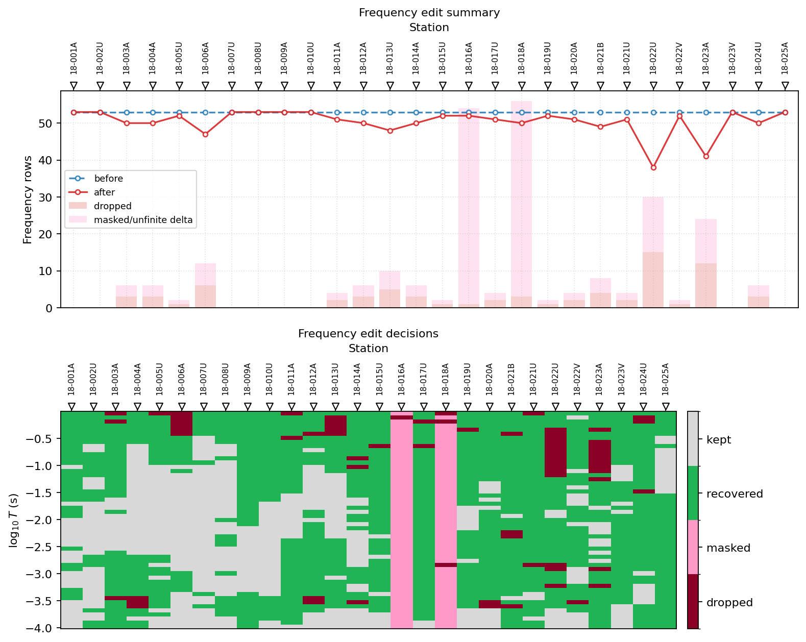
If the decision plot is dominated by recovered or masked colors, the edit is not conservative and should be justified.

Regrid To A Target Grid

Use regrid_to when you already have the target frequencies.

import numpy as np

from pycsamt.emtools.frequency import regrid_to

target_freq = np.array([1.0, 3.0, 10.0, 30.0, 100.0, 300.0, 1000.0])

regridded = regrid_to(
    "data/AMT/WILLY_DATA/L18PLT",
    target_freq,
    method="linear",
    inplace=False,
)

method controls interpolation behavior. The implementation supports nearest-neighbor and log-frequency interpolation paths used by the module’s helpers. Use a target grid that is meaningful for your inversion or comparison, not merely convenient.

Build A Log-Spaced Grid

Use regrid_logspace to generate a grid automatically.

from pycsamt.emtools.frequency import regrid_logspace

regular = regrid_logspace(
    "data/AMT/WILLY_DATA/L18PLT",
    fmin=1.0,
    fmax=10000.0,
    per_decade=6,
    method="linear",
    inplace=False,
)

band_hz=(lo, hi) is accepted as an alias for fmin and fmax. n_per_decade is accepted as an alias for per_decade when per_decade is left at its default.

Decimation And Moving Average Smoothing

Use decimate_step to keep every step row. Use smooth_mavg to apply a moving average along frequency.

from pycsamt.emtools.frequency import decimate_step, smooth_mavg

decimated = decimate_step(
    "data/AMT/WILLY_DATA/L18PLT",
    step=2,
    inplace=False,
)

smoothed = smooth_mavg(
    "data/AMT/WILLY_DATA/L18PLT",
    k=3,
    on="z",
    inplace=False,
)

Smoothing changes the measured tensor values. Use it as a processing choice, not as a plotting convenience, and report the window size.

Align Station Grids

Use align_grid when stations need a common grid.

from pycsamt.emtools.frequency import align_grid

union_aligned = align_grid(
    "data/AMT/WILLY_DATA/L18PLT",
    mode="union",
    method="nearest",
)

intersection_aligned = align_grid(
    "data/AMT/WILLY_DATA/L18PLT",
    mode="intersection",
    method="nearest",
)

ref_aligned = align_grid(
    "data/AMT/WILLY_DATA/L18PLT",
    mode="ref",
    ref_station="18-001A",
    method="nearest",
)

The modes are:

Mode	Meaning
union	Use all frequencies present in any station.
intersection	Use only frequencies present in every station.
ref	Use the grid from ref_station.

intersection can be empty or nearly empty for independently processed data because frequencies may not match bit-for-bit. If the intersection is empty, the function returns the input sites unchanged.

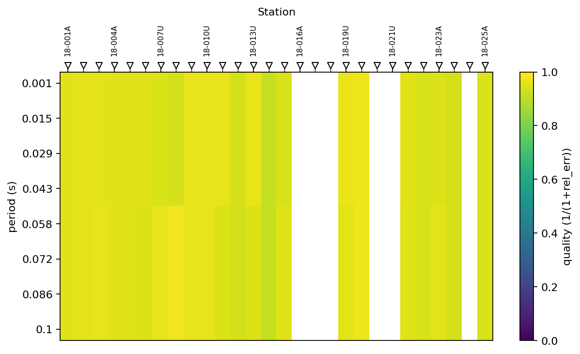
Coverage And Quality Heatmap

plot_coverage_quality_heatmap shows which station-frequency cells exist and how reliable they are according to relative impedance error.

import matplotlib.pyplot as plt

from pycsamt.emtools.frequency import plot_coverage_quality_heatmap

fig, ax = plt.subplots(figsize=(9, 4.5))
plot_coverage_quality_heatmap(
    "data/AMT/WILLY_DATA/L18PLT",
    axis="period",
    ax=ax,
)
fig.tight_layout()

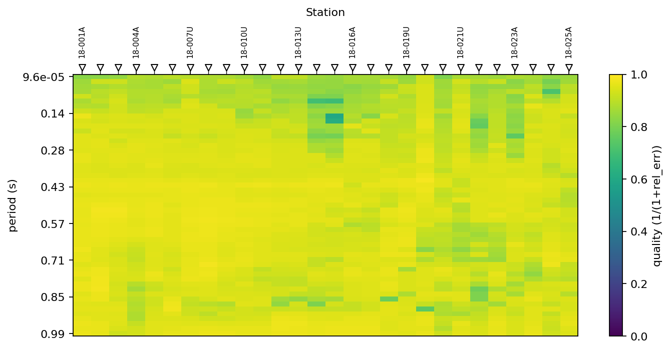
The color is 1 / (1 + relative_error). Values closer to 1 are higher quality. Missing cells indicate no frequency row on the union grid for that station.

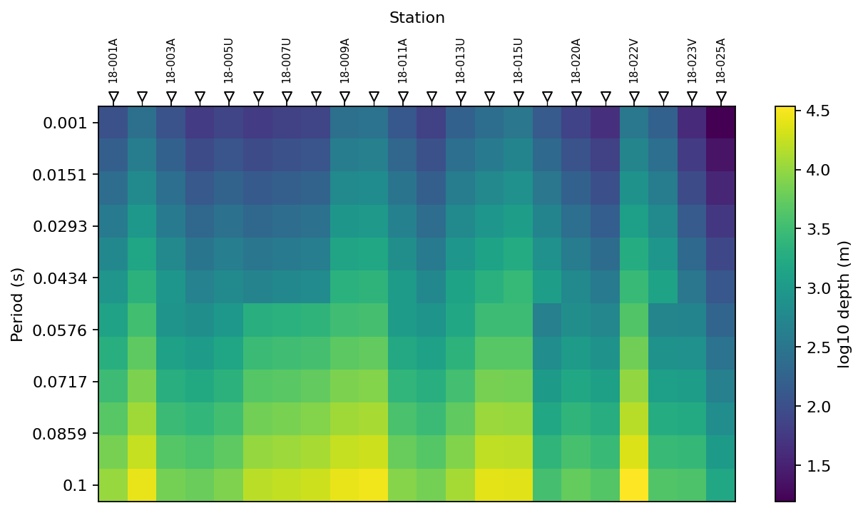
Apparent Depth Pseudo-Section

plot_apparent_depth_psection converts determinant apparent resistivity and frequency into a skin-depth-style apparent depth:

\[depth \approx 503 \sqrt{\rho / f}\]

import matplotlib.pyplot as plt

from pycsamt.emtools.frequency import plot_apparent_depth_psection

fig, ax = plt.subplots(figsize=(9, 4.5))
plot_apparent_depth_psection(
    "data/AMT/WILLY_DATA/L18PLT",
    axis_y="period",
    agg="median",
    log_color=True,
    ax=ax,
)
fig.tight_layout()

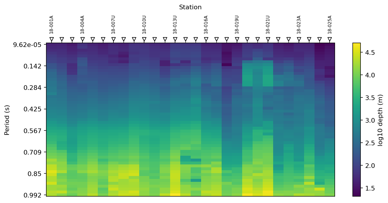
This is a diagnostic visualization, not an inversion result. Use it to see how apparent depth varies across stations and periods.

Band Microstrips

plot_band_microstrips collapses periods into bands and plots three summary metrics per station and band:

• median log10 determinant apparent resistivity;

• median determinant phase;

• median tipper amplitude when available.

import matplotlib.pyplot as plt

from pycsamt.emtools.frequency import plot_band_microstrips

bands = [
    (1e-4, 1e-3),
    (1e-3, 1e-2),
    (1e-2, 1e-1),
    (1e-1, 1.0),
]

fig, ax = plt.subplots(figsize=(9, 6))
plot_band_microstrips(
    "data/AMT/WILLY_DATA/L18PLT",
    bands=bands,
    ax=ax,
)
fig.tight_layout()

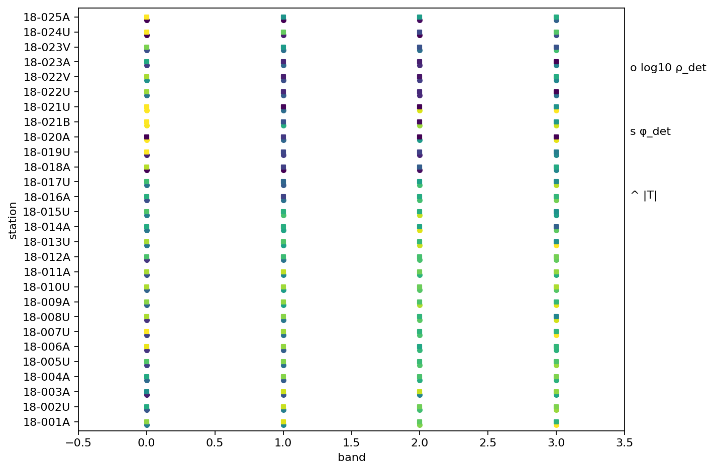
Use microstrips for compact survey summaries. They are not a substitute for full curves when a band contains strong internal variation.

Recommended Processing Pattern

A conservative frequency workflow looks like this:

1. Inspect the native frequency range and confidence table.

2. Select a physically meaningful band.

3. Decide whether bad rows should be dropped, masked, or recovered.

4. Save the edit report and decision table.

5. Regrid or align only when the next workflow requires it.

6. Plot coverage and apparent depth after editing.

7. Keep the original data available for audit.

from pathlib import Path

import matplotlib.pyplot as plt

from pycsamt.emtools.frequency import (
    edit_frequencies_by_confidence,
    plot_apparent_depth_psection,
    plot_coverage_quality_heatmap,
    regrid_logspace,
    select_band,
)

survey = "data/AMT/WILLY_DATA/L18PLT"
out = Path("outputs/frequency_l18plt")
out.mkdir(parents=True, exist_ok=True)

banded = select_band(survey, fmin=10.0, fmax=1000.0)
result = edit_frequencies_by_confidence(
    banded,
    mode="recover",
    before_sites=banded,
    ci_hi=0.72,
    ci_lo=0.50,
    reject="drop",
    api=False,
)
regular = regrid_logspace(result.sites, fmin=10.0, fmax=1000.0, per_decade=6)

result.report.to_csv(out / "frequency_edit_report.csv", index=False)
result.decisions.to_csv(out / "frequency_edit_decisions.csv", index=False)

fig1, ax1 = plt.subplots(figsize=(9, 4.5))
plot_coverage_quality_heatmap(regular, ax=ax1)
fig1.savefig(out / "coverage_quality_heatmap.png", dpi=200)

fig2, ax2 = plt.subplots(figsize=(9, 4.5))
plot_apparent_depth_psection(regular, ax=ax2)
fig2.savefig(out / "apparent_depth_psection.png", dpi=200)

Common Failure Modes

Using default ci_hi without checking confidence

Recovery needs trusted rows at or above ci_hi. If the survey confidence never reaches that value, recovery cannot behave as expected.

Dropping rows before checking downstream needs

Dropping shortens the grid. If the next step expects aligned grids, masking may be safer.

Masking rows before plotting finite-only workflows

Some workflows ignore or fail on NaN rows. Save a decision table so missing values are explainable.

Regridding too early

Interpolation can hide native acquisition problems. Inspect native confidence first.

Empty intersection alignment

Independently processed stations may have no exact shared frequency. Use union or a reference station when appropriate.

Smoothing as hidden preprocessing

Moving averages change tensor values. Report the window and apply it intentionally.

Worked Example

The gallery example uses L18PLT from data/AMT/WILLY_DATA/ and brings in KAP03 for heterogeneous-grid alignment. It demonstrates band selection, confidence editing, recovery, reports, decision plots, regridding, decimation, smoothing, grid alignment, coverage heatmaps, apparent-depth pseudo-sections, and band microstrips.

Open the rendered example here: Frequency editing, resampling, and QC (pycsamt.emtools.frequency).