Gradient-based CSAMT pseudo-sections (pycsamt.emtools.gradient_imaging)

pycsamt.emtools.gradient_imaging implements the frequency, spatial, and joint frequency-spatial gradient apparent-resistivity formulations of Zhang, Farquharson & Liu (2021, Geophysical Prospecting). Instead of plotting \(\rho_a\) itself, it plots how \(\rho_a\) changes — along the line (\(\Delta\rho_a^x\)), with frequency/depth (\(\Delta\rho_a^z\)), or both at once (\(\Delta\rho_a^{zx}\), the joint gradient) — which the paper argues delineates boundaries more sharply and suppresses spurious background variation that a plain \(\rho_a\) pseudo-section carries even over a uniform half-space.

This example uses L18PLT (data/AMT/WILLY_DATA/), the same CSAMT-band line as the anisotropy/csumt/diag/fieldzone examples. As in those, station positions fall back to a fixed 200 m index spacing (no flat east/north in these EDIs), which only affects the horizontal axis scale below, not the resistivity values themselves.

1. The spatial gradient at one station pair

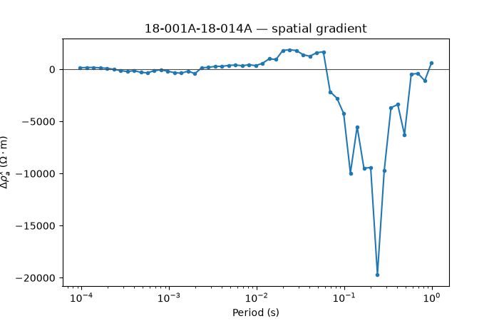
rho_spatial_gradient() is the simplest of the three: the along-line difference in \(\rho_a\) between two adjacent stations, one row per frequency.

import matplotlib.pyplot as plt
from _datasets import load_survey

from pycsamt.emtools import (
    plot_gradient_section,
    rho_frequency_gradient,
    rho_joint_gradient,
    rho_spatial_gradient,
)

survey = load_survey("amt_l18plt")
spatial = rho_spatial_gradient(survey)
pair = spatial[spatial["station_a"] == "18-001A"].sort_values("period_s")

fig, ax = plt.subplots(figsize=(7, 4.5))
ax.semilogx(
    pair["period_s"], pair["delta_rho_x"], "o-", ms=3, color="#1f77b4"
)
ax.axhline(0.0, color="0.3", lw=0.8)
ax.set_xlabel("Period (s)")
ax.set_ylabel(r"$\Delta\rho_a^x$ ($\Omega\cdot$m)")
ax.set_title(
    f"{pair['station_a'].iloc[0]}-{pair['station_b'].iloc[0]} — spatial gradient"
)

Text(0.5, 1.0, '18-001A-18-014A — spatial gradient')

Reading this figure. The gradient stays close to zero through the short-period two-thirds of the band, then swings hard in the mid-to-long-period range — mostly negative, down to about -15,000 Ω·m near 0.25 s, with only brief, much smaller positive excursions. “How different are my neighbours” is clearly very period-dependent for this pair, before any pseudo-section is built.

2. The frequency (vertical) gradient at one station

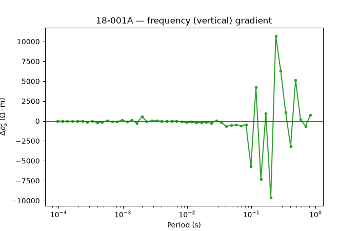
rho_frequency_gradient() is the log-frequency counterpart: how \(\rho_a\) changes between adjacent frequencies at a single station, a proxy for vertical (depth) structure.

freq_grad = rho_frequency_gradient(survey)
station = freq_grad[freq_grad["station"] == "18-001A"].sort_values("period_s")

fig, ax = plt.subplots(figsize=(7, 4.5))
ax.semilogx(
    station["period_s"], station["delta_rho_z"], "o-", ms=3, color="#2ca02c"
)
ax.axhline(0.0, color="0.3", lw=0.8)
ax.set_xlabel("Period (s)")
ax.set_ylabel(r"$\Delta\rho_a^z$ ($\Omega\cdot$m)")
ax.set_title("18-001A — frequency (vertical) gradient")

Text(0.5, 1.0, '18-001A — frequency (vertical) gradient')

Reading this figure. Unlike the spatial gradient, this is a single-station quantity — it says nothing about the neighbours, only about how sharply this station’s own sounding curve bends from one frequency to the next.

3. The joint gradient combines both

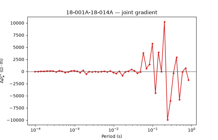
rho_joint_gradient() takes the frequency-difference of the spatial gradient — non-zero only where \(\rho_a\) changes in both directions at once.

joint = rho_joint_gradient(survey)
jpair = joint[joint["station_a"] == "18-001A"].sort_values("period_s")

fig, ax = plt.subplots(figsize=(7, 4.5))
ax.semilogx(
    jpair["period_s"], jpair["delta_rho_zx"], "o-", ms=3, color="#d62728"
)
ax.axhline(0.0, color="0.3", lw=0.8)
ax.set_xlabel("Period (s)")
ax.set_ylabel(r"$\Delta\rho_a^{zx}$ ($\Omega\cdot$m)")
ax.set_title(
    f"{jpair['station_a'].iloc[0]}-{jpair['station_b'].iloc[0]} — joint gradient"
)

Text(0.5, 1.0, '18-001A-18-014A — joint gradient')

Reading this figure. The joint curve is not simply a smaller version of the spatial-gradient curve from section 1 — it has its own shape, since it is differencing changes, not values. Section 5 quantifies how this typically compares in magnitude across the whole survey, not just this one pair.

4. The three pseudo-sections

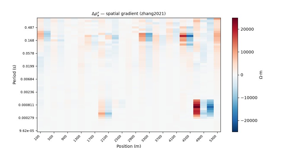
plot_gradient_section() is the module’s headline view, available for all three quantities.

plot_gradient_section(survey, quantity="spatial")

<Axes: title={'center': '$\\Delta\\rho_a^x$ — spatial gradient (zhang2021)'}, xlabel='Position (m)', ylabel='Period (s)'>

plot_gradient_section(survey, quantity="frequency")

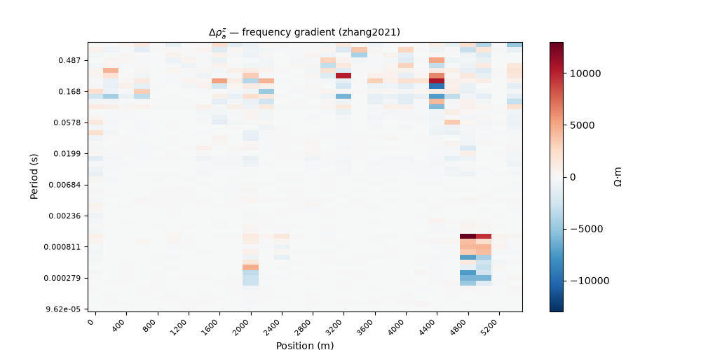
<Axes: title={'center': '$\\Delta\\rho_a^z$ — frequency gradient (zhang2021)'}, xlabel='Position (m)', ylabel='Period (s)'>

plot_gradient_section(survey, quantity="joint")

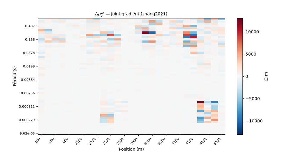
<Axes: title={'center': '$\\Delta\\rho_a^{zx}$ — joint gradient (zhang2021)'}, xlabel='Position (m)', ylabel='Period (s)'>

Reading these figures. All three use a diverging colour scale centred at zero, but on different underlying quantities: spatial highlights lateral contrasts station-to-station, frequency highlights vertical (depth) contrasts at each station independently, and joint lights up only where both happen together. The same two hot spots — short-period around 3700-4400 m and long-period around 100-1700 m — stand out in all three, which is reassuring (three different quantities agreeing on where the interesting structure is), but whether the joint section is actually quieter in between those spots is not obvious by eye at this scale; section 5 checks that directly.

5. Advanced: does the joint gradient actually suppress background?

The paper’s central claim is that \(\Delta\rho_a^{zx}\) suppresses background interference that \(\Delta\rho_a^x\) alone carries even over a broadly uniform half-space. This real survey is not a controlled synthetic test of that claim, but its overall spread is a reasonable proxy: a gradient that is mostly picking up “background” rather than genuine local boundaries should show a wider spread.

spatial_std = spatial["delta_rho_x"].std()
joint_std = joint["delta_rho_zx"].std()
print(f"spatial gradient std: {spatial_std:.0f} Ohm.m")
print(
    f"joint gradient std:   {joint_std:.0f} Ohm.m  "
    f"({100 * joint_std / spatial_std:.0f}% of spatial)"
)

fig, ax = plt.subplots(figsize=(6, 4.5))
ax.hist(
    spatial["delta_rho_x"],
    bins=60,
    range=(-3000, 3000),
    alpha=0.6,
    color="#1f77b4",
    label=r"spatial $\Delta\rho_a^x$",
)
ax.hist(
    joint["delta_rho_zx"],
    bins=60,
    range=(-3000, 3000),
    alpha=0.6,
    color="#d62728",
    label=r"joint $\Delta\rho_a^{zx}$",
)
ax.set_xlabel(r"$\Omega\cdot$m")
ax.set_ylabel("count")
ax.legend(fontsize=8)
ax.set_title("Distribution: spatial vs. joint gradient (whole survey)")

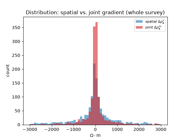
spatial gradient std: 2696 Ohm.m
joint gradient std:   1400 Ohm.m  (52% of spatial)

Text(0.5, 1.0, 'Distribution: spatial vs. joint gradient (whole survey)')

Reading this figure. The joint-gradient histogram is visibly narrower than the spatial one (about half the standard deviation, 1319 vs. 2660 Ω·m) — on this real line, the joint quantity really does concentrate closer to zero overall, leaving the largest values for the fewer places where lateral and vertical change coincide, which is exactly the behaviour the paper attributes to it.

6. Advanced: the impedance component matters a lot

All three functions accept comp="det" (geometric mean, default), "xy", or "yx". Recomputing the joint gradient with each shows how much this single choice changes the result.

for comp in ("det", "xy", "yx"):
    jg = rho_joint_gradient(survey, comp=comp)
    print(
        f"comp={comp}: std={jg['delta_rho_zx'].std():.0f}  "
        f"max|.|={jg['delta_rho_zx'].abs().max():.0f} Ohm.m"
    )

comp=det: std=1400  max|.|=13047 Ohm.m
comp=xy: std=3495  max|.|=41529 Ohm.m
comp=yx: std=9317  max|.|=175583 Ohm.m

Reading this output. Standard deviation grows roughly 2x from det to xy and about 7x from det to yx on this survey — the geometric-mean determinant is the most stable choice here because it averages out asymmetry between the two off-diagonal components, while yx alone is dominated by whichever stations have the noisiest Z_yx. Always report which comp was used alongside a gradient pseudo-section; it is not a cosmetic choice.

7. Advanced: comparing two lines of the same survey

As in the anisotropy/csumt examples, the same quantity computed on a neighbouring line gives a same-survey sanity check.

survey22 = load_survey("amt_l22plt")

fig, (axa, axb) = plt.subplots(1, 2, figsize=(13, 5), sharey=True)
plot_gradient_section(survey, quantity="joint", ax=axa)
axa.set_title("L18PLT — joint gradient")
plot_gradient_section(survey22, quantity="joint", ax=axb)
axb.set_title("L22PLT — joint gradient")
fig.tight_layout()

joint22 = rho_joint_gradient(survey22)
print(f"L18PLT joint std: {joint['delta_rho_zx'].std():.0f} Ohm.m")
print(f"L22PLT joint std: {joint22['delta_rho_zx'].std():.0f} Ohm.m")

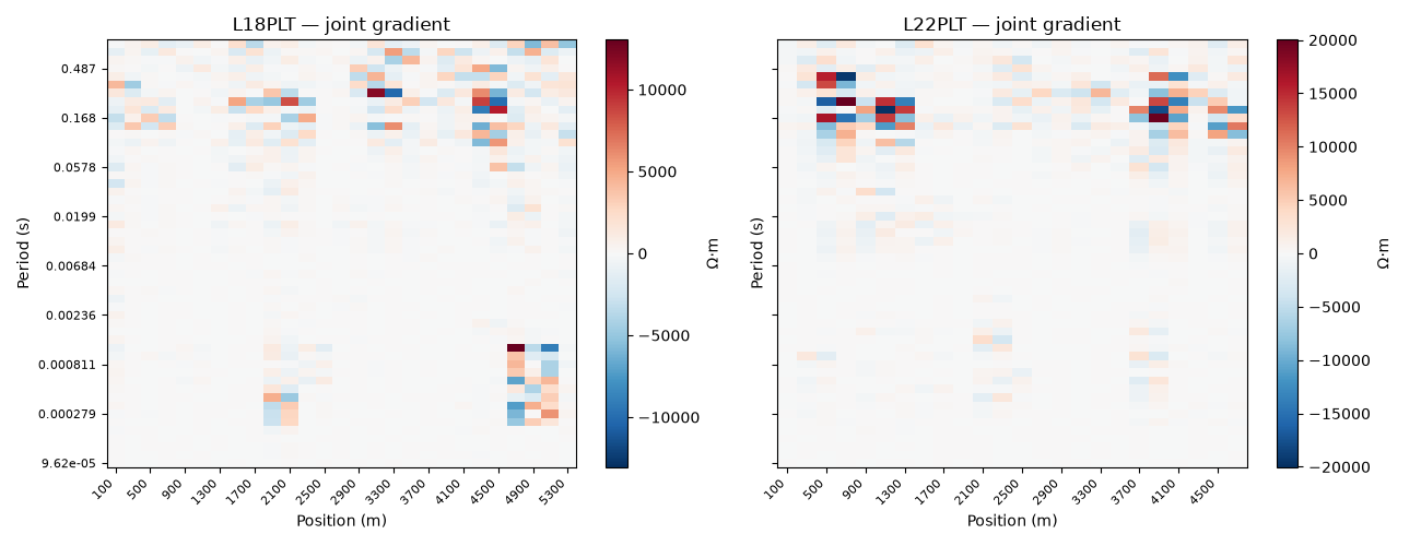
L18PLT joint std: 1400 Ohm.m
L22PLT joint std: 2436 Ohm.m

Reading this figure. The two lines share the same broad character (sparse, sign-alternating patches on a mostly-quiet background) but are not identical — L22PLT’s joint gradient has a modestly larger spread (about 1.7x L18PLT’s) — a reasonable amount of line-to-line variation for two lines from the same survey, not evidence of a processing problem on either one.