Impedance-Tensor Diagnostics

pycsamt.emtools.impedance gives direct views of the complex impedance tensor before it is reduced to apparent resistivity, phase, phase-tensor attributes, dimensionality classes, or inversion input. Use this page when you want to look at the tensor itself and ask:

• do Zxy and Zyx behave like an approximately antisymmetric 1-D/2-D response?

• are diagonal terms small compared with off-diagonal terms?

• does one station have a different complex trajectory from its neighbours?

• is the determinant response stable enough to trust as a compact rotationally invariant summary?

Full callable signatures live in the API reference. This page focuses on interpretation, concrete workflows, and code.

What The Module Uses

All public functions normalize their input through ensure_sites. That means the same call can accept a directory of EDI files, an existing Sites object, an EDICollection, or EDI-like objects. Each station must expose a complex impedance array shaped (n_frequency, 2, 2) and a frequency array.

The tensor components are indexed as:

\[\begin{split}Z = \begin{bmatrix} Z_{xx} & Z_{xy} \\ Z_{yx} & Z_{yy} \end{bmatrix}.\end{split}\]

The diagnostics on this page use Z directly. That is important: apparent resistivity and phase are derived products, while the phasor wheel, antisymmetry residual, and determinant track keep the complex tensor visible.

Load A Survey Once

Use ensure_sites first when you are building a notebook or script. That makes the rest of the code explicit and avoids reloading files for each plot.

from pathlib import Path

from pycsamt.emtools import ensure_sites

edi_dir = Path("data/AMT/WILLY_DATA/L18PLT")
survey = ensure_sites(
    edi_dir,
    recursive=True,
    on_dup="replace",
    strict=True,
    verbose=1,
)

strict=True is useful in documentation, tests, and reproducible analysis because it fails early when no valid sites are found. In an interactive exploratory session you may prefer strict=False so an empty or partly broken directory can still be inspected.

Choose The Right Diagnostic

The three public views answer different questions.

View	Best Question	Main Output
phasor wheel	How do selected complex tensor components move with period at one station?	A polar Argand-style plot for one station.
antisymmetry residual	Where along the line do Zxy and Zyx stop cancelling as a 1-D/2-D response would suggest?	A station-period pseudo-section.
determinant track	Is a compact rotationally invariant station response stable, and how wide is its uncertainty band?	Magnitude and phase curves versus period.

The views are complementary. The phasor wheel is local and visual, the residual pseudo-section is survey-wide, and the determinant track is a station-level summary.

The Phasor Wheel

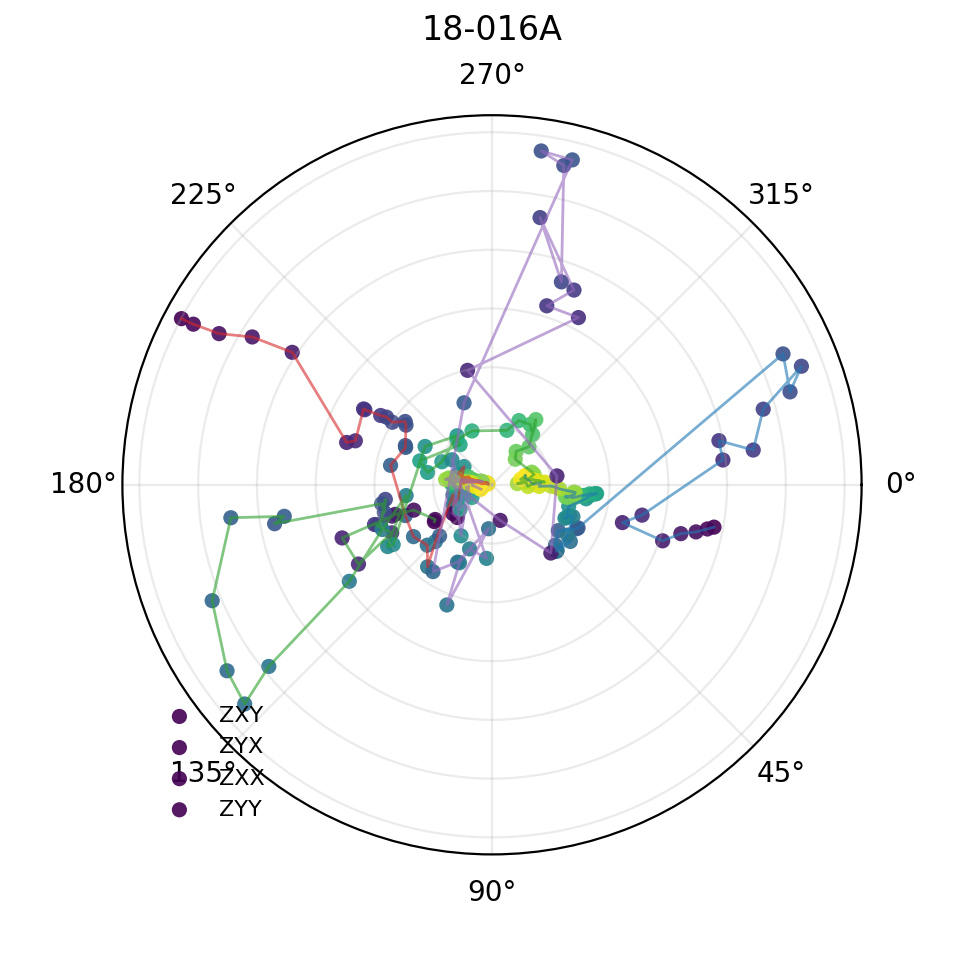
plot_phasor_wheel draws selected impedance components as complex phasors. For each frequency sample, the component phase becomes the polar angle and the component magnitude becomes the radius. Colour encodes log-period, so a station becomes a period-ordered complex trajectory.

import matplotlib.pyplot as plt

from pycsamt.emtools import ensure_sites
from pycsamt.emtools.impedance import plot_phasor_wheel

survey = ensure_sites("data/AMT/WILLY_DATA/L18PLT", strict=True)

ax = plot_phasor_wheel(
    survey,
    station="18-001A",
    components=("xy", "yx"),
    radius="abs",
    connect=True,
    figsize=(5.0, 5.0),
)

ax.figure.savefig("phasor_wheel_18-001A.png", dpi=200)
plt.close(ax.figure)

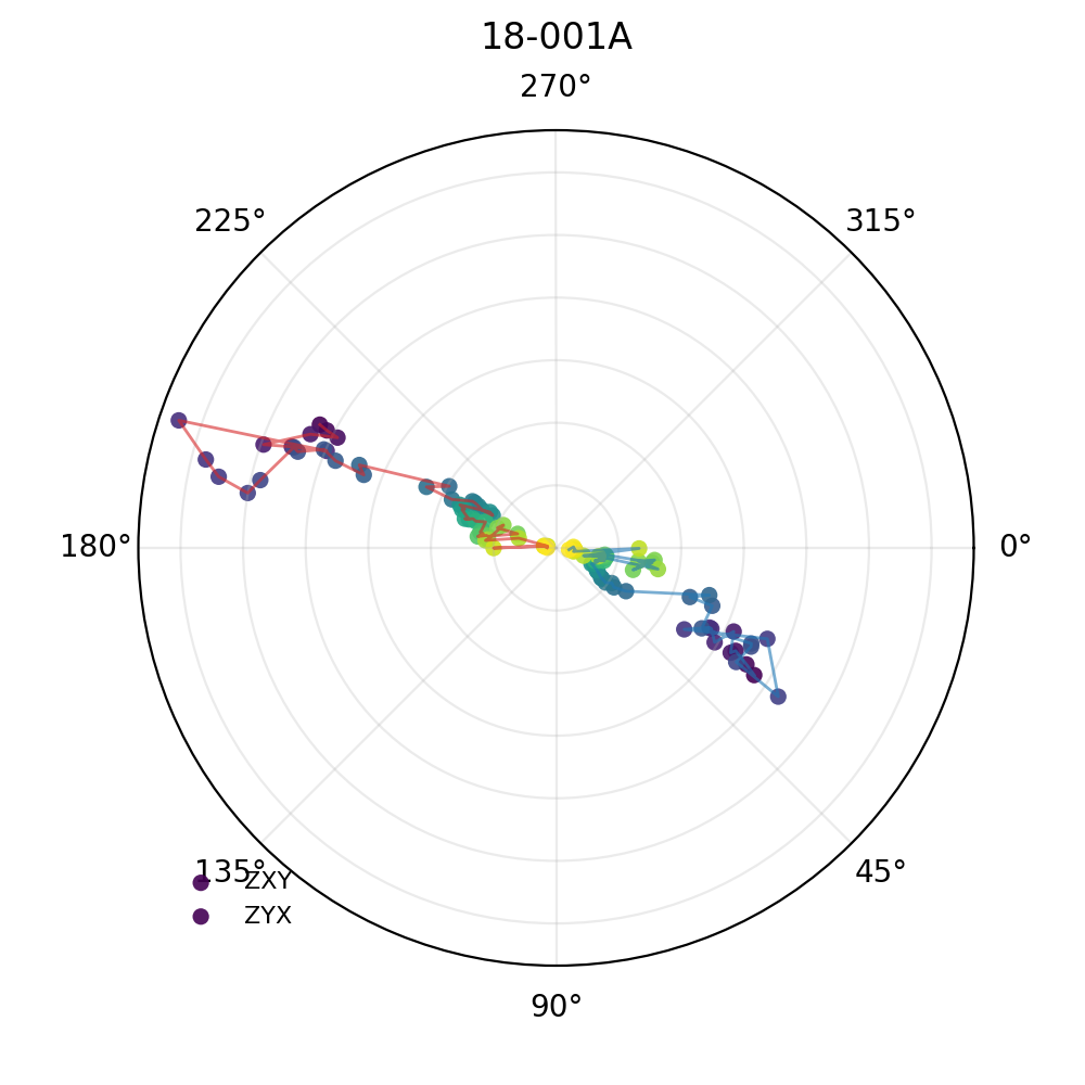
Read this plot as a direct complex-plane diagnostic. If Zxy and Zyx are close to a clean 1-D/2-D off-diagonal pair, their phasors should be broadly opposite in phase, because the ideal relation is Zxy ~= -Zyx. If the two arcs bend into different sectors, cross, or change separation with period, the station is telling you that one simple dimensional picture is probably not enough.

Use Period Bands

The pband argument selects a period interval in seconds. This is a simple way to ask whether shallow and deeper parts of the sounding have different tensor behaviour.

import matplotlib.pyplot as plt

from pycsamt.emtools import ensure_sites
from pycsamt.emtools.impedance import plot_phasor_wheel

survey = ensure_sites("data/AMT/WILLY_DATA/L18PLT", strict=True)
station = "18-001A"

fig, axes = plt.subplots(
    1,
    2,
    figsize=(9.5, 5.0),
    subplot_kw={"polar": True},
)

plot_phasor_wheel(
    survey,
    station=station,
    pband=(9e-5, 1e-3),
    ax=axes[0],
)
axes[0].set_title("short periods")

plot_phasor_wheel(
    survey,
    station=station,
    pband=(1e-1, 1.0),
    ax=axes[1],
)
axes[1].set_title("long periods")

fig.tight_layout()
fig.savefig("phasor_period_bands_18-001A.png", dpi=200)
plt.close(fig)

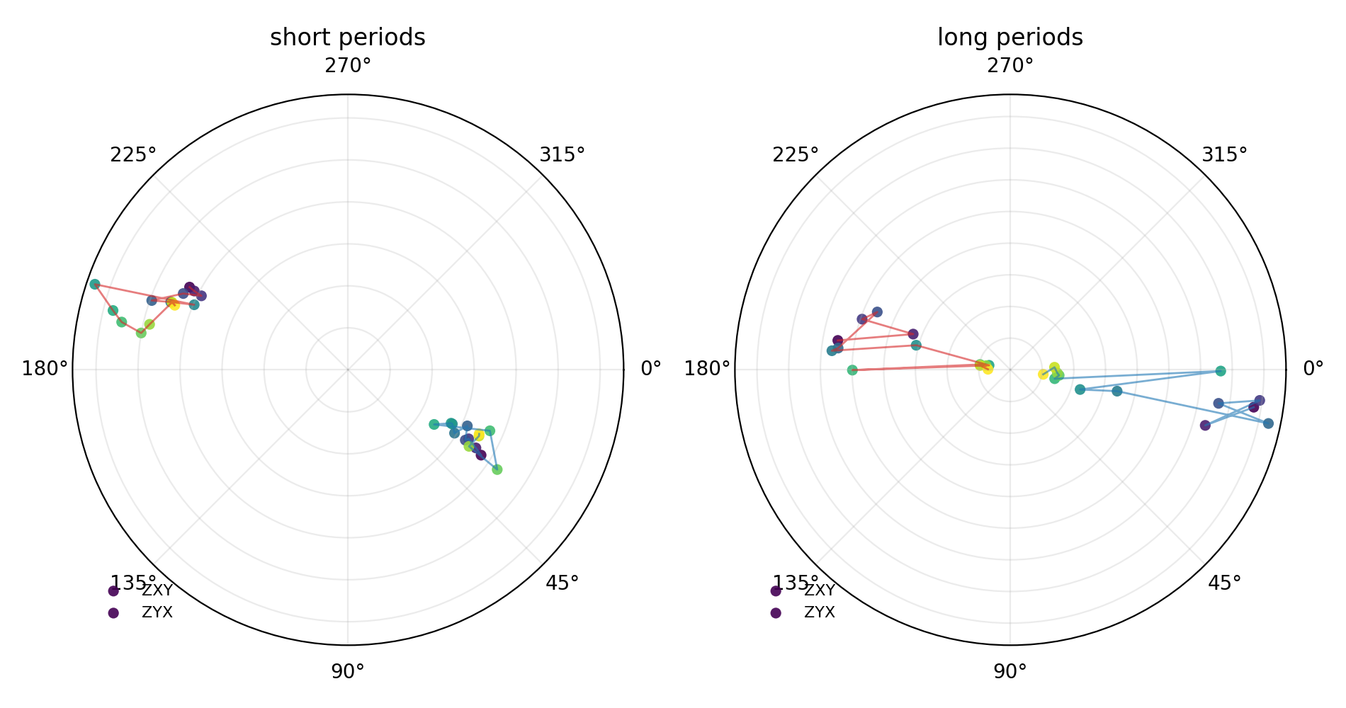
If the short-period and long-period arcs have the same shape but different radii, the main change is magnitude. If they rotate into different angular sectors or the xy and yx relation changes, the complex response itself is changing with period.

Include The Diagonal Terms

For a simple 1-D earth, the diagonal tensor components are ideally zero. For a 2-D earth in the correct strike coordinate system, the off-diagonal terms dominate. In field data, Zxx and Zyy rarely vanish exactly, but their size relative to Zxy and Zyx is still informative.

from pycsamt.emtools import ensure_sites
from pycsamt.emtools.impedance import plot_phasor_wheel

survey = ensure_sites("data/AMT/WILLY_DATA/L18PLT", strict=True)

ax = plot_phasor_wheel(
    survey,
    station="18-001A",
    components=("xy", "yx", "xx", "yy"),
    radius="norm",
    connect=False,
    ms=2.5,
)

ax.figure.savefig("phasor_all_components_18-001A.png", dpi=200)

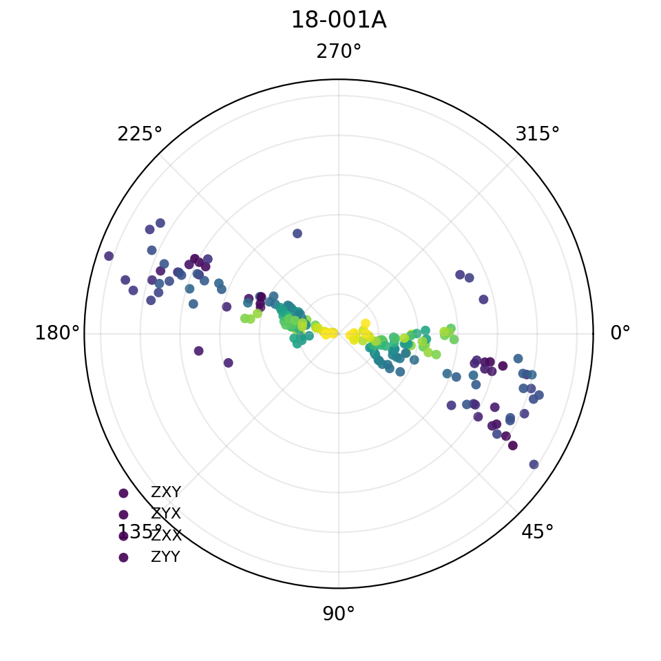
radius="norm" scales each component radius by a robust component magnitude, which helps when one component would otherwise dominate the display. Use radius="abs" when you need the physical size relation to remain visible.

Compute Component Magnitudes

The plot is useful, but a station report should also write the numbers. The lower-level helper _get_z_block returns the validated tensor and frequency arrays used by the plotting functions.

import numpy as np

from pycsamt.emtools import ensure_sites
from pycsamt.emtools._core import _get_z_block, _iter_items, _name

survey = ensure_sites("data/AMT/WILLY_DATA/L18PLT", strict=True)

rows = []
for index, site in enumerate(_iter_items(survey)):
    _, z, freq = _get_z_block(site)
    if z is None:
        continue

    rows.append(
        {
            "station": _name(site, index),
            "mean_abs_zxx": float(np.nanmean(np.abs(z[:, 0, 0]))),
            "mean_abs_zxy": float(np.nanmean(np.abs(z[:, 0, 1]))),
            "mean_abs_zyx": float(np.nanmean(np.abs(z[:, 1, 0]))),
            "mean_abs_zyy": float(np.nanmean(np.abs(z[:, 1, 1]))),
        }
    )

for row in rows[:5]:
    print(row)

{'station': '18-001A', 'mean_abs_zxx': 446.87532535812795, 'mean_abs_zxy': 808.4345401982367, 'mean_abs_zyx': 1145.0965447882752, 'mean_abs_zyy': 557.6049786167763}
{'station': '18-002U', 'mean_abs_zxx': 133.0926461161051, 'mean_abs_zxy': 620.1474584088546, 'mean_abs_zyx': 859.6134726088661, 'mean_abs_zyy': 257.84731425866534}
{'station': '18-003A', 'mean_abs_zxx': 109.30601909208245, 'mean_abs_zxy': 610.4449839811526, 'mean_abs_zyx': 388.2097256381032, 'mean_abs_zyy': 106.6560768811014}
{'station': '18-004A', 'mean_abs_zxx': 252.91269027986166, 'mean_abs_zxy': 839.1242870947025, 'mean_abs_zyx': 681.5954183841726, 'mean_abs_zyy': 300.46444606989644}
{'station': '18-005U', 'mean_abs_zxx': 202.61429236412803, 'mean_abs_zxy': 811.4948595592589, 'mean_abs_zyx': 563.3054411247073, 'mean_abs_zyy': 261.3767440473993}

This is not meant to replace phase-tensor dimensionality or skew analysis. It is a quick tensor sanity check: if the diagonal terms are large at a station, look at dimensionality, distortion, static shift, and strike diagnostics before treating that station as simple 2-D input.

Off-Diagonal Antisymmetry

plot_offdiag_antisym_residual maps how far the off-diagonal components depart from the ideal cancellation relation:

\[r = {|Z_{xy} + Z_{yx}| \over |Z_{xy}| + |Z_{yx}| + \epsilon}.\]

The implementation clips the result to 0 <= r <= 1. Values near zero mean the off-diagonal terms cancel well. Larger values mean the two off-diagonal terms are less antisymmetric.

import matplotlib.pyplot as plt

from pycsamt.emtools import ensure_sites
from pycsamt.emtools.impedance import plot_offdiag_antisym_residual

survey = ensure_sites("data/AMT/WILLY_DATA/L18PLT", strict=True)

fig, ax = plt.subplots(figsize=(10.0, 4.8))
plot_offdiag_antisym_residual(
    survey,
    vlim=0.8,
    cmap="magma",
    ax=ax,
)
ax.set_title("L18PLT off-diagonal antisymmetry residual")

fig.tight_layout()
fig.savefig("offdiag_antisymmetry_l18plt.png", dpi=200)
plt.close(fig)

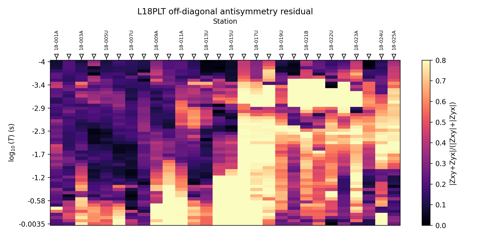
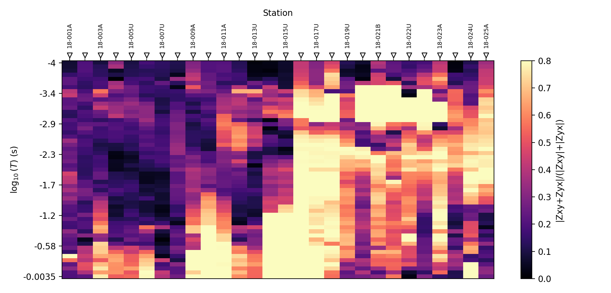
The horizontal axis is station order. The vertical axis is log10(period). Warm columns mark stations or period bands where Zxy and Zyx fail to cancel. That does not prove a particular geology by itself, but it is a strong cue to compare against phase-tensor skew, anisotropy ratio, induction arrows, and nearby lines.

Rank Stations By Residual

The pseudo-section shows the pattern. A table names the stations.

import numpy as np
import pandas as pd

from pycsamt.emtools import ensure_sites
from pycsamt.emtools._core import _get_z_block, _iter_items, _name

survey = ensure_sites("data/AMT/WILLY_DATA/L18PLT", strict=True)

rows = []
for index, site in enumerate(_iter_items(survey)):
    _, z, freq = _get_z_block(site)
    if z is None:
        continue

    xy = np.abs(z[:, 0, 1])
    yx = np.abs(z[:, 1, 0])
    residual = np.abs(z[:, 0, 1] + z[:, 1, 0]) / (xy + yx + 1e-24)
    residual = np.clip(residual, 0.0, 1.0)

    rows.append(
        {
            "station": _name(site, index),
            "mean_residual": float(np.nanmean(residual)),
            "p90_residual": float(np.nanpercentile(residual, 90)),
            "max_residual": float(np.nanmax(residual)),
            "n_frequency": int(np.isfinite(residual).sum()),
        }
    )

ranking = (
    pd.DataFrame(rows)
    .sort_values("mean_residual", ascending=False)
    .reset_index(drop=True)
)

print(ranking.head(10))
ranking.to_csv("impedance_antisymmetry_ranking.csv", index=False)

   station  mean_residual  p90_residual  max_residual  n_frequency
0  18-016A       0.786452      0.942456      0.958245           53
1  18-018A       0.749186      0.961107      0.998407           53
2  18-017U       0.715415      0.877221      0.920305           53
3  18-023A       0.640977      0.860594      0.957943           53
4  18-021B       0.623736      0.964924      0.990659           53
5  18-021U       0.556974      0.968757      0.980216           53
6  18-022U       0.538863      0.873291      0.963180           53
7  18-024U       0.526460      0.811147      0.961759           53
8  18-015U       0.500570      0.984507      0.999133           53
9  18-025A       0.498164      0.782128      0.842395           53

Use mean_residual for a broad station ranking. Use p90_residual when you want to highlight stations with a persistent high-residual tail. Use max_residual only as a trigger for manual inspection because one bad frequency can dominate it.

Compare With Anisotropy Or Skew

The antisymmetry residual is related to, but not identical with, diagonal skew or apparent anisotropy. The best practice is to compare metrics instead of assuming they flag the same stations.

import numpy as np
import pandas as pd

from pycsamt.emtools import anisotropy_table, ensure_sites
from pycsamt.emtools._core import _get_z_block, _iter_items, _name

survey = ensure_sites("data/AMT/WILLY_DATA/L18PLT", strict=True)

residual_rows = []
for index, site in enumerate(_iter_items(survey)):
    _, z, freq = _get_z_block(site)
    if z is None:
        continue

    xy = np.abs(z[:, 0, 1])
    yx = np.abs(z[:, 1, 0])
    residual = np.abs(z[:, 0, 1] + z[:, 1, 0]) / (xy + yx + 1e-24)
    residual_rows.append(
        {
            "station": _name(site, index),
            "antisym_mean": float(np.nanmean(np.clip(residual, 0.0, 1.0))),
        }
    )

residual_df = pd.DataFrame(residual_rows).set_index("station")
aniso_df = anisotropy_table(survey).set_index("station")

merged = residual_df.join(
    aniso_df[["mean_swift_skew", "mean_ratio_log10"]],
    how="inner",
)
merged["abs_ratio_log10"] = merged["mean_ratio_log10"].abs()

print(merged.corr(numeric_only=True))

                  antisym_mean  ...  abs_ratio_log10
antisym_mean          1.000000  ...         0.719606
mean_swift_skew      -0.592220  ...        -0.613406
mean_ratio_log10      0.631375  ...         0.886388
abs_ratio_log10       0.719606  ...         1.000000

[4 rows x 4 columns]

When correlations are strong, the diagnostics are probably responding to a shared tensor feature. When they disagree, inspect the stations manually. A station can have a high skew because of diagonal terms but still have off-diagonal components that nearly cancel.

Determinant Track

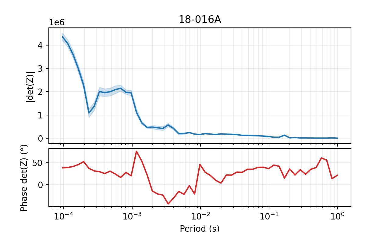
plot_determinant_track summarizes a station with the determinant of the full impedance tensor:

\[\det(Z) = Z_{xx} Z_{yy} - Z_{xy} Z_{yx}.\]

The plot has two panels: |det(Z)| and determinant phase versus period. If impedance errors are available as z_err, pyCSAMT draws a Monte Carlo uncertainty band for the determinant magnitude.

import matplotlib.pyplot as plt

from pycsamt.emtools import ensure_sites
from pycsamt.emtools.impedance import plot_determinant_track

survey = ensure_sites("data/AMT/WILLY_DATA/L18PLT", strict=True)

fig = plot_determinant_track(
    survey,
    station="18-016A",
    pband=(1e-4, 1.0),
    pcts=(10.0, 50.0, 90.0),
    n_draws=300,
    figsize=(6.8, 4.2),
)

fig.savefig("determinant_track_18-016A.png", dpi=200)
plt.close(fig)

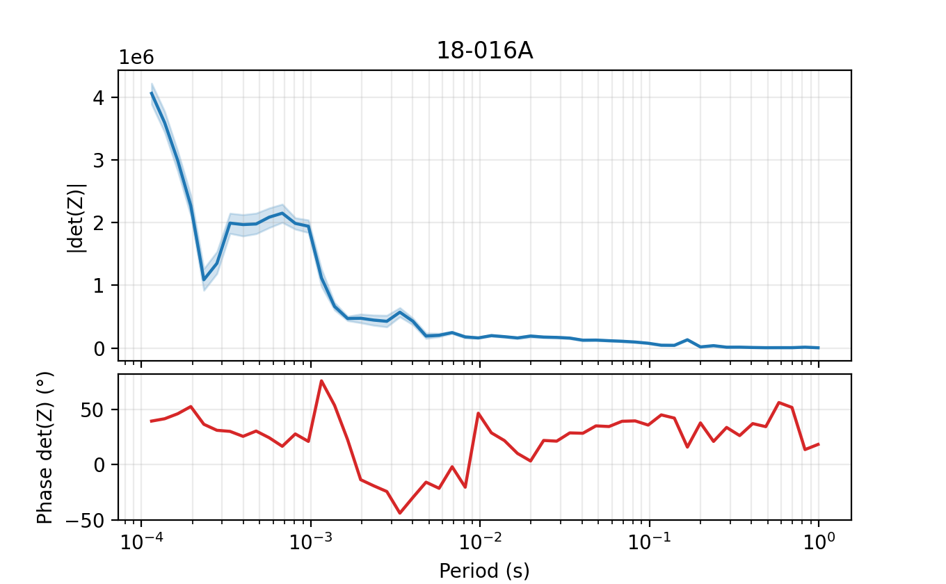
The default percentile band is the 10th to 90th percentile interval. Increase n_draws when you need a smoother band. Keep seed fixed only if you call the lower-level determinant helper directly and need bit-for-bit reproducibility in a report.

Compare Two Stations

The determinant track is most useful when compared across stations with contrasting tensor diagnostics.

import matplotlib.pyplot as plt

from pycsamt.emtools import ensure_sites
from pycsamt.emtools.impedance import plot_determinant_track

survey = ensure_sites("data/AMT/WILLY_DATA/L18PLT", strict=True)

fig = plt.figure(figsize=(11.0, 4.8))
grid = fig.add_gridspec(
    2,
    2,
    height_ratios=(2, 1),
    hspace=0.08,
    wspace=0.25,
)

left_axes = (fig.add_subplot(grid[0, 0]), fig.add_subplot(grid[1, 0]))
right_axes = (fig.add_subplot(grid[0, 1]), fig.add_subplot(grid[1, 1]))

plot_determinant_track(survey, station="18-016A", axes=left_axes)
plot_determinant_track(survey, station="18-007U", axes=right_axes)

left_axes[0].set_title("high residual station")
right_axes[0].set_title("low residual station")

fig.savefig("determinant_station_comparison.png", dpi=200)
plt.close(fig)

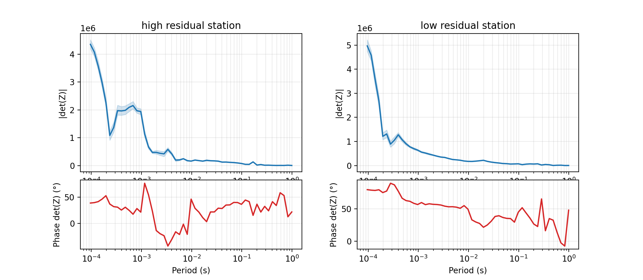
Look for differences in curve smoothness, phase wrapping, band width, and period-local instability. A wide uncertainty band does not automatically make the station unusable, but it should lower your confidence in interpretations that depend on small determinant features.

Measure Determinant Band Width

For reports, compute a simple relative band-width number instead of judging the shaded region by eye.

import numpy as np
import pandas as pd

from pycsamt.emtools import ensure_sites
from pycsamt.emtools._core import _get_z_block, _iter_items, _name
from pycsamt.emtools.impedance import _det_ci

survey = ensure_sites("data/AMT/WILLY_DATA/L18PLT", strict=True)

rows = []
for index, site in enumerate(_iter_items(survey)):
    _, z, freq, z_err = _get_z_block(site, with_errors=True)
    if z is None:
        continue

    mag, phase, band = _det_ci(
        z,
        freq,
        z_err,
        pcts=(10.0, 50.0, 90.0),
        n_draws=300,
        seed=0,
    )
    relative_width = (band[:, 1] - band[:, 0]) / (mag + 1e-24)

    rows.append(
        {
            "station": _name(site, index),
            "median_det_abs": float(np.nanmedian(mag)),
            "median_relative_band_width": float(
                np.nanmedian(relative_width)
            ),
            "max_relative_band_width": float(np.nanmax(relative_width)),
        }
    )

det_quality = (
    pd.DataFrame(rows)
    .sort_values("median_relative_band_width", ascending=False)
    .reset_index(drop=True)
)

print(det_quality.head(10))
det_quality.to_csv("determinant_band_width.csv", index=False)

   station  median_det_abs  median_relative_band_width  max_relative_band_width
0  18-021U   138059.459579                    1.244798                 1.558835
1  18-020A    58591.215698                    0.981629                 1.719329
2  18-021B   304870.766789                    0.675971                 1.572428
3  18-022V    54687.185702                    0.414231                 1.390426
4  18-018A    12533.221781                    0.286987                 1.416562
5  18-022U    59346.090486                    0.272911                 1.511982
6  18-025A    22893.891856                    0.259362                 1.010240
7  18-013U   409823.995492                    0.242223                 1.320911
8  18-024U    37132.445937                    0.241634                 0.978317
9  18-023A    57853.829945                    0.223259                 1.416815

The private helper _det_ci is used here because it exposes the computed arrays behind the public plot. For stable production code, prefer the public plotting function unless you need these exact numbers.

Compare Neighbouring Lines

A warm residual column is more meaningful when the same style of feature appears on neighbouring survey lines or when it lines up with known geology. Use the same colour limit when comparing lines.

import matplotlib.pyplot as plt

from pycsamt.emtools import ensure_sites
from pycsamt.emtools.impedance import plot_offdiag_antisym_residual

line18 = ensure_sites("data/AMT/WILLY_DATA/L18PLT", strict=True)
line22 = ensure_sites("data/AMT/WILLY_DATA/L22PLT", strict=True)

fig, axes = plt.subplots(1, 2, figsize=(13.0, 5.0), sharey=True)

plot_offdiag_antisym_residual(line18, vlim=0.8, ax=axes[0])
axes[0].set_title("L18PLT")

plot_offdiag_antisym_residual(line22, vlim=0.8, ax=axes[1])
axes[1].set_title("L22PLT")

fig.tight_layout()
fig.savefig("antisymmetry_line_comparison.png", dpi=200)
plt.close(fig)

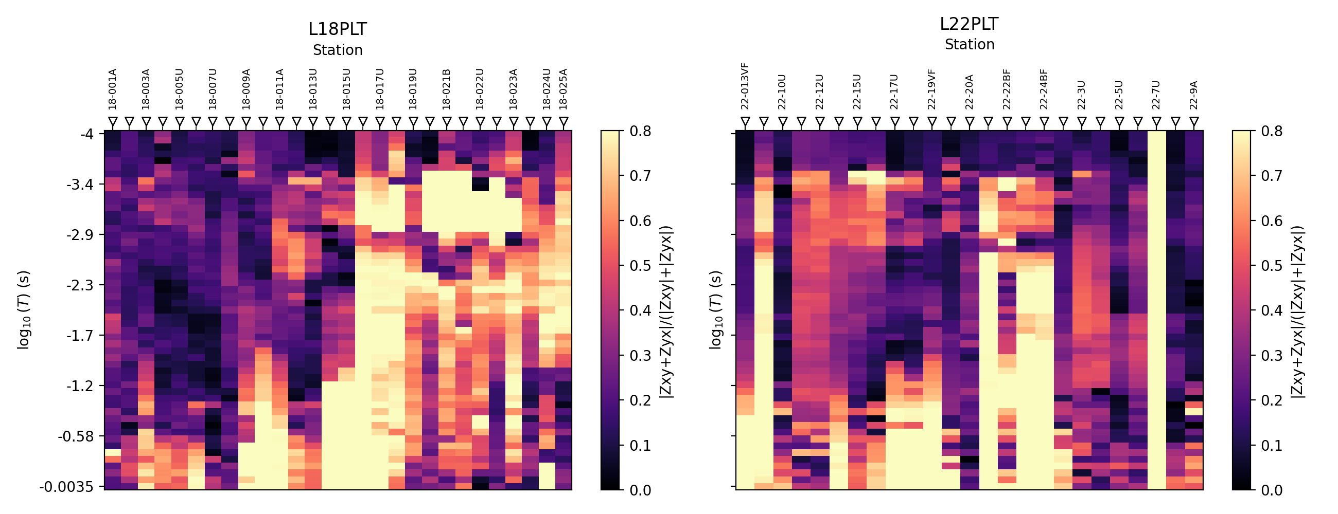
If one line is uniformly warmer, check acquisition quality, processing settings, coordinate orientation, and frequency coverage before making a geological claim. If a localized warm zone repeats across lines, it is more likely to represent real structure or a persistent distortion effect.

Common Interpretation Checks

Use these checks before promoting an impedance diagnostic into an interpretation:

Zxy and Zyx do not cancel

Compare against phase-tensor skew, Swift skew, anisotropy ratio, and induction arrows. The residual is a warning flag, not a complete dimensionality classifier.

Diagonal components are large

Inspect whether the coordinate frame is appropriate. If a 2-D strike rotation is justified, rotate before concluding that the response is strongly 3-D.

Only one frequency is anomalous

Treat it as a possible processing or data-quality issue. Cross-check with QC and frequency-editing tools.

The determinant band is wide

Check whether z_err is realistic and whether the station has noisy or sparse frequency samples.

The phasor wheel is hard to read

Use pband to split the period range and components to reduce clutter. Use radius="norm" when component magnitudes differ too much for one display.

Saving A Reproducible Bundle

The following script writes the main impedance outputs for one survey: one residual pseudo-section, one station ranking, one phasor wheel, and one determinant track.

from pathlib import Path

import matplotlib.pyplot as plt
import numpy as np
import pandas as pd

from pycsamt.emtools import ensure_sites
from pycsamt.emtools._core import _get_z_block, _iter_items, _name
from pycsamt.emtools.impedance import (
    plot_determinant_track,
    plot_offdiag_antisym_residual,
    plot_phasor_wheel,
)

out = Path("impedance_report_l18plt")
out.mkdir(parents=True, exist_ok=True)

survey = ensure_sites("data/AMT/WILLY_DATA/L18PLT", strict=True)

fig, ax = plt.subplots(figsize=(10.0, 4.8))
plot_offdiag_antisym_residual(survey, vlim=0.8, ax=ax)
fig.tight_layout()
fig.savefig(out / "antisymmetry_residual.png", dpi=200)
plt.close(fig)

rows = []
for index, site in enumerate(_iter_items(survey)):
    _, z, freq = _get_z_block(site)
    if z is None:
        continue
    xy = np.abs(z[:, 0, 1])
    yx = np.abs(z[:, 1, 0])
    residual = np.clip(
        np.abs(z[:, 0, 1] + z[:, 1, 0]) / (xy + yx + 1e-24),
        0.0,
        1.0,
    )
    rows.append(
        {
            "station": _name(site, index),
            "mean_residual": float(np.nanmean(residual)),
            "p90_residual": float(np.nanpercentile(residual, 90)),
        }
    )

ranking = pd.DataFrame(rows).sort_values(
    "mean_residual",
    ascending=False,
)
ranking.to_csv(out / "antisymmetry_ranking.csv", index=False)

station = ranking.iloc[0]["station"]

ax = plot_phasor_wheel(
    survey,
    station=station,
    components=("xy", "yx", "xx", "yy"),
    radius="norm",
)
ax.figure.savefig(out / f"phasor_{station}.png", dpi=200)
plt.close(ax.figure)

fig = plot_determinant_track(survey, station=station, n_draws=300)
fig.savefig(out / f"determinant_{station}.png", dpi=200)
plt.close(fig)

Worked Example

The gallery example applies the same ideas to bundled WILLY survey lines and connects the impedance views with anisotropy rankings.

Open the rendered gallery page here: Impedance-tensor diagnostics (pycsamt.emtools.impedance).