Phase-tensor and Bahr skew diagnostics (pycsamt.emtools.skew)

pycsamt.emtools.skew measures how far a station departs from a simple 1-D/2-D structure using two independent skew formulas — the classic Bahr (1988) invariant \(\eta\) computed directly from \(Z\), and the Caldwell-Bibby-Bahr phase-tensor skew angle \(\beta\) (via pycsamt.emtools.tensor) — then offers several ways to mask, trim, or vote on frequencies where that skew is acceptably low. This example uses L18PLT (data/AMT/WILLY_DATA/), the same line the qc example already flagged as high_skew at every one of its 28 stations under a strict default threshold. That finding is not a fluke: this whole page traces its consequences through every skew-based masking function in the module.

1. Simple: the skew table

skew_table() is a thin wrapper around pycsamt.emtools.tensor.build_phase_tensor_table(), returning one row per (station, frequency) with the phase-tensor skew angle \(\beta\) (column skew, identical to column beta).

import matplotlib.pyplot as plt
import numpy as np
from _datasets import load_survey

from pycsamt.emtools import (
    bahr_skewness,
    close_skew_gaps,
    ensure_sites,
    keep_longest_low_skew,
    mask_by_skew,
    plot_skew_percentile_ribbon,
    plot_skew_traffic_psection,
    plot_skew_vote_band,
    plot_skewness,
    select_low_skew_band,
    skew_table,
)
from pycsamt.emtools._core import (
    _get_z_block,
    _iter_items,
    _name,
)

survey = load_survey("amt_l18plt")

table = skew_table(survey)
abs_skew = table["skew"].abs()
print(abs_skew.describe())

by_station = table.groupby("station")["skew"].apply(
    lambda s: s.abs().median()
)
print("lowest-skew stations:\n", by_station.sort_values().head(3))
print("highest-skew stations:\n", by_station.sort_values().tail(3))

count    1484.000000
mean       44.536824
std        25.198206
min         0.353578
25%        23.593647
50%        40.992429
75%        66.994007
max        89.910303
Name: skew, dtype: float64
lowest-skew stations:
 station
18-015U    22.459269
18-017U    22.912833
18-016A    23.525350
Name: skew, dtype: float64
highest-skew stations:
 station
18-018A    66.547818
18-022V    66.787861
18-023A    67.022970
Name: skew, dtype: float64

Reading this output. Median \(|\beta|\) across all 1484 station-frequency rows is 41.0 degrees, mean 44.5 — this is the same survey the qc example flagged high_skew at every station under its strict default threshold, now seen directly at the source. Even the lowest-median station, 18-015U, still runs 22.5 degrees. Two stations threaded through earlier examples land at opposite ends here: 18-016A (flagged for extreme ratio anisotropy) is actually among the least skewed (23.5), while 18-018A (also flagged for ratio anisotropy) is among the most skewed (66.5) — a reminder that ratio anisotropy and phase-tensor skew measure genuinely different things, even when the same stations get flagged by both.

2. Bahr skewness: an independent formula

bahr_skewness() computes the classic Bahr (1988) invariant \(\eta\) straight from the complex impedance tensor — no phase-tensor decomposition involved — and plot_skewness() plots it against a 2D/3D threshold.

s = ensure_sites(survey, recursive=False)
z_by_name = {}
for i, ed in enumerate(_iter_items(s)):
    name = _name(ed, i)
    if name in ("18-016A", "18-018A"):
        _, z, fr = _get_z_block(ed)
        z_by_name[name] = (z, fr)

fig, axes = plt.subplots(1, 2, figsize=(11.0, 4.2))
for ax, name in zip(axes, ("18-016A", "18-018A")):
    z, fr = z_by_name[name]
    eta = bahr_skewness(z)
    print(
        f"{name}: Bahr eta min/median/max = "
        f"{np.nanmin(eta):.2f} / {np.nanmedian(eta):.2f} / {np.nanmax(eta):.2f}"
    )
    plot_skewness(fr, z, threshold=0.4, ax=ax, title=name)

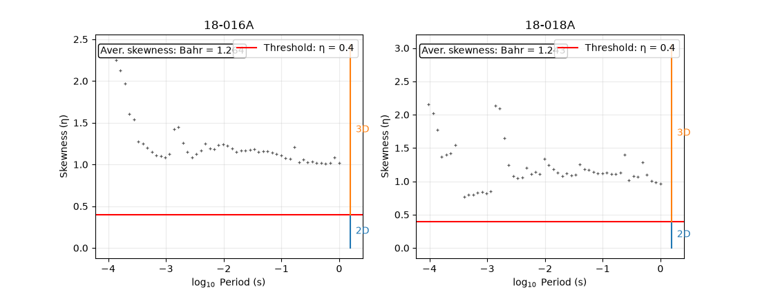
18-016A: Bahr eta min/median/max = 1.01 / 1.16 / 2.34
18-018A: Bahr eta min/median/max = 0.76 / 1.12 / 2.92

Reading this output/figure. Bahr’s classic threshold is \(\eta=0.4\) (below: acceptably 2D; above: 3D or noise/distortion dominated) — every single point for both stations sits above it, and the “2D” wedge on the right of each panel is essentially unused. But the two stations’ average Bahr skewness is nearly identical (1.26 vs. 1.25) despite their very different phase-tensor \(\beta\) medians from section 1 (23.5 vs. 66.5 degrees) — the two independent skew formulas agree that both stations are unambiguously non-2D, but disagree sharply on which one is “worse”. Neither number is wrong; they simply weight the tensor’s asymmetry differently, a real reason to check more than one skew diagnostic before ranking stations by structural complexity.

3. Masking by skew threshold

mask_by_skew() sets rows with \(|\beta|\) above (or, in other modes, below) a threshold to NaN.

import logging  # noqa: E402

logging.disable(logging.ERROR)
masked_default = mask_by_skew(survey, thresh=6.0)
masked_loose = mask_by_skew(survey, thresh=45.0)
logging.disable(logging.NOTSET)


def n_finite(sites, name):
    ss = ensure_sites(sites, recursive=False)
    for i, ed in enumerate(_iter_items(ss)):
        if _name(ed, i) == name:
            _, z, fr = _get_z_block(ed)
            return int(np.isfinite(z).all(axis=(1, 2)).sum()), z.shape[0]
    raise KeyError(name)


for name in ("18-001A", "18-016A", "18-018A"):
    kept_d, total = n_finite(masked_default, name)
    kept_l, _ = n_finite(masked_loose, name)
    print(
        f"{name}: thresh=6 (default) keeps {kept_d}/{total};  thresh=45 keeps {kept_l}/{total}"
    )

18-001A: thresh=6 (default) keeps 2/53;  thresh=45 keeps 22/53
18-016A: thresh=6 (default) keeps 5/53;  thresh=45 keeps 40/53
18-018A: thresh=6 (default) keeps 1/53;  thresh=45 keeps 9/53

Reading this output. At the module’s default thresh=6, almost nothing survives — 2-6 of 53 frequencies per station, matching section 1’s finding that even the calmest station sits at 22.5 degrees median. Raising the threshold to 45 (close to this survey’s mean) recovers a much more usable fraction, without needing to fabricate cleaner data: the function works exactly as documented, the default is simply tuned for a far less skewed survey than this one.

4. Keeping only the longest low-skew run

keep_longest_low_skew() finds the longest contiguous run of low-skew frequencies and masks everything else — unless no run reaches min_len, in which case it falls back to fallback ("keep_all" by default).

logging.disable(logging.ERROR)
for name in ("18-016A", "18-018A"):
    kept_strict, total = n_finite(
        keep_longest_low_skew(survey, thresh=25.0, min_len=5),
        name,
    )
    print(f"{name}: thresh=25, min_len=5 keeps {kept_strict}/{total}")
logging.disable(logging.NOTSET)

18-016A: thresh=25, min_len=5 keeps 16/53
18-018A: thresh=25, min_len=5 keeps 53/53

Reading this output. 18-016A (this survey’s calmer station) genuinely gets trimmed to its longest acceptable run: 16 of 53 frequencies. 18-018A (the most skewed) keeps all 53 — not because it passed, but because no contiguous run of 5 or more low-skew frequencies exists anywhere in its spectrum, so the fallback quietly returns everything unmasked. This is worth checking explicitly before trusting a “kept everything” result: on a station this skewed, that outcome means the threshold could not be satisfied at all, not that the station is clean.

5. Closing small gaps in the low-skew mask

close_skew_gaps() fills short interior gaps (up to max_gap frequencies) inside an otherwise-passing stretch, rather than fragmenting it into many tiny kept segments.

logging.disable(logging.ERROR)
for name in ("18-001A", "18-016A", "18-018A"):
    k0, total = n_finite(
        close_skew_gaps(survey, thresh=25.0, max_gap=0), name
    )
    k3, _ = n_finite(close_skew_gaps(survey, thresh=25.0, max_gap=3), name)
    print(
        f"{name}: max_gap=0 keeps {k0}/{total};  max_gap=3 keeps {k3}/{total}"
    )
logging.disable(logging.NOTSET)

18-001A: max_gap=0 keeps 8/53;  max_gap=3 keeps 12/53
18-016A: max_gap=0 keeps 30/53;  max_gap=3 keeps 33/53
18-018A: max_gap=0 keeps 2/53;  max_gap=3 keeps 2/53

Reading this output. Allowing gaps of up to 3 frequencies recovers a handful of extra rows for 18-001A (8 → 12) and 18-016A (30 → 33) — short interior dips above threshold get bridged rather than splitting one usable stretch into several. 18-018A stays at 2 of 53 either way: with so few passing points to begin with, there is no run long enough for gap-filling to help.

6. Survey-wide voting on a shared low-skew band

select_low_skew_band() first restricts each station to its own longest acceptable run, then keeps only the frequencies where at least frac of stations agree.

logging.disable(logging.ERROR)
for frac in (0.6, 0.3, 0.1):
    band = select_low_skew_band(survey, thresh=30.0, frac=frac, min_len=3)
    ss = ensure_sites(band, recursive=False)
    total = kept = 0
    for i, ed in enumerate(_iter_items(ss)):
        _, z, fr = _get_z_block(ed)
        total += z.shape[0]
        kept += int(np.isfinite(z).all(axis=(1, 2)).sum())
    print(
        f"frac={frac}: kept {kept}/{total} station-frequency rows survey-wide"
    )
logging.disable(logging.NOTSET)

frac=0.6: kept 0/1484 station-frequency rows survey-wide
frac=0.3: kept 308/1484 station-frequency rows survey-wide
frac=0.1: kept 924/1484 station-frequency rows survey-wide

Reading this output. At frac=0.6 — a 60% majority of the 28 stations agreeing station-by-station on their own longest run — nothing survives at all: not one frequency reaches that bar anywhere in the survey, because each station’s acceptable stretch sits at different frequencies. Lowering the bar to 30% recovers 308 of 1484 rows (~21%); 10% recovers 924 (~62%). This is an honest, if severe, consequence of how heterogeneous the skew is station to station on this particular line, not a malfunction.

7. Three “beautiful” survey-wide skew views

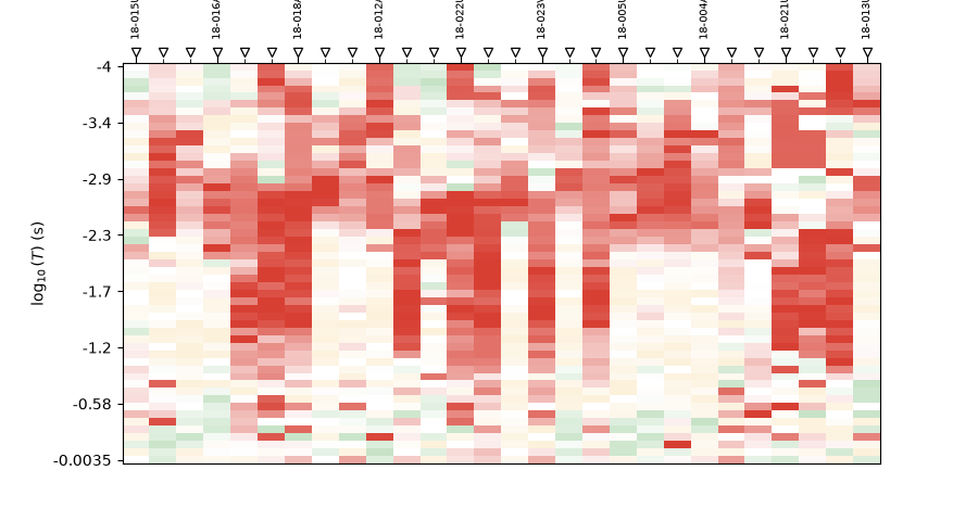
plot_skew_traffic_psection() colours every (station, period) cell green/amber/red by \(|\beta|\), with alpha encoding confidence (distance from the nearest threshold).

plot_skew_traffic_psection(survey, t1=15.0, t2=35.0)

<Axes: xlabel='Station', ylabel='$\\log_{10}(T)$ (s)'>

Reading this figure. With thresholds relaxed to this survey’s own scale (\(t_1=15\), \(t_2=35\), rather than the function’s textbook defaults of 3/6 which would render this entire section solid red), the survey-wide split is 13% green, 30% amber, 57% red — red dominates but is not everything. The contrast is sharpest between neighboring columns: 18-018A (this page’s most-skewed station) is 92% red with almost no amber or green, while its neighbor 18-016A is only 28% red against 28% green and 43% amber — visibly calmer, exactly matching the station ranking from section 1.

plot_skew_percentile_ribbon(survey)

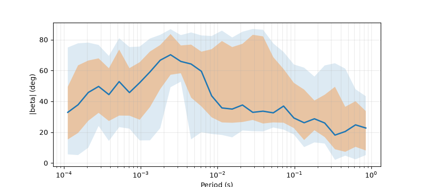
<Axes: xlabel='Period (s)', ylabel='|beta| (deg)'>

Reading this figure. The median \(|\beta|\) curve (solid line) runs 20-70 degrees across the whole period range, with the 25th-75th percentile band (darker) and 10th-90th (lighter) both staying well clear of zero everywhere — there is no period band on this line where skew drops to a classically “safe” level for any meaningful fraction of stations.

plot_skew_vote_band(survey, thresh=30.0)

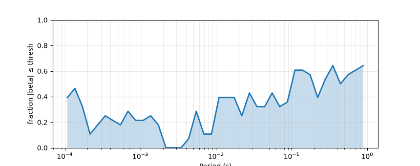
<Axes: xlabel='Period (s)', ylabel='fraction |beta| ≤ thresh'>

Reading this figure. The fraction of stations with \(|\beta|\le 30\) per period bin mostly sits under 0.5, dipping to zero around \(10^{-3}\) s and only climbing above 0.6 at the longest periods on the right edge.

8. Advanced: two different “votes” are not the same number

Section 7’s vote-band curve touches ~0.6-0.65 at the longest periods — so why did section 6’s select_low_skew_band(frac=0.6) keep nothing? plot_skew_vote_band() votes on the raw, pointwise \(|\beta|\le\text{thresh}\) condition alone. select_low_skew_band() votes on whether each frequency falls inside that station’s own longest contiguous run — a strictly narrower condition that can (and here does) push every station’s vote down at once, even at periods where its raw skew was briefly fine.

from pycsamt.emtools import (
    build_phase_tensor_table,  # noqa: E402
)

pt = build_phase_tensor_table(survey, recursive=False)
p = pt["period"].to_numpy(dtype=float)
b = pt["skew"].abs().to_numpy(dtype=float)
lp = np.log10(np.maximum(p, 1e-9))
tail = lp >= np.percentile(lp, 90)
raw_vote_tail = float(np.nanmean(b[tail] <= 30.0))
print(
    f"raw pointwise fraction |beta|<=30 in the longest-period decile: {raw_vote_tail:.2f}"
)

raw pointwise fraction |beta|<=30 in the longest-period decile: 0.62

Reading this output. The raw pointwise fraction in the longest periods is comfortably above 0.6, matching section 7’s vote-band curve — confirming the two functions really do disagree for the documented reason (one extra restriction to each station’s own best contiguous run) rather than a bug in either. Choosing between them matters in practice: plot_skew_vote_band() is the right diagnostic for “how much of the survey is clean at this period”, while select_low_skew_band() is the right masking function when what is actually needed is one shared, contiguous band usable across the whole line.