Note

Go to the end to download the full example code.

CSAMT source overprint and near-field effects (`pycsamt.emtools.source_effects`)#

pycsamt.emtools.source_effects quantifies how the artificial CSAMT transmitter contaminates a sounding, using two independent formulas from two different papers: the Yan & Fu (2004) / Da et al. (2016) ground-wave/surface-wave amplitude ratio $\beta_{Ey}$ (a source-overprint index, threshold 3%), and the Wang & Lin (2023) skin-depth field-zone classification with a near-field correction built on the equatorial HED transfer function $F(p)$. Unlike natural-source MT, CSAMT needs the source-receiver offset $r$ to evaluate either formula. This example uses real pycsamt.emtools.fieldzone-style data: the same ten-station Tongkeng CSAMT line (data/CSAMT) used in the fieldzone example, with its real ~1 km transmitter offset and the same 1170 $\Omega\cdot\mathrm{m}$ far-field-only representative resistivity derived there.

1. The core concept: how $\beta_{Ey}$ depends on offset#

overprint_beta() is pure arithmetic – no sites needed. At fixed resistivity, sweeping frequency at three representative offsets (the same trio used in the fieldzone example) shows the expected physical trend: a closer transmitter pushes the “safe” (low $\beta$) frequency band down.

import matplotlib.pyplot as plt
import numpy as np

from pycsamt.emtools import (
    BETA_THRESH_PCT,
    correct_near_field,
    detect_source_overprint,
    normalize_response,
    overprint_beta,
    plot_normalized_response,
    plot_overprint_section,
    source_overprint_table,
)

freq_sweep = np.logspace(-1, 3, 60)
fig, ax = plt.subplots(figsize=(7.5, 4.2))
for offset, color in zip(
    [500.0, 1000.0, 4000.0], ["#d62728", "#ff7f0e", "#2ca02c"]
):
    beta = overprint_beta(rho=1170.0, freq=freq_sweep, offset=offset)
    ax.loglog(freq_sweep, beta, color=color, label=f"r={offset:g} m")
    above = freq_sweep[beta > BETA_THRESH_PCT]
    if above.size:
        print(
            f"offset={offset:g} m: beta>{BETA_THRESH_PCT:g}% for f up to {above.max():.3g} Hz"
        )
ax.axhline(
    BETA_THRESH_PCT,
    color="0.3",
    ls="--",
    lw=1,
    label=f"threshold {BETA_THRESH_PCT:g}%",
)
ax.set_xlabel("Frequency (Hz)")
ax.set_ylabel(r"$\beta_{Ey}$ (%)")
ax.set_title(r"$\beta_{Ey}$ vs. frequency at $\rho$=1170 $\Omega\cdot$m")
ax.grid(True, which="both", alpha=0.25)
ax.legend(fontsize=8)

$$\beta_{Ey}$ vs. frequency at $\rho$=1170 $\Omega\cdot$m$

offset=500 m: beta>3% for f up to 1e+03 Hz
offset=1000 m: beta>3% for f up to 1e+03 Hz
offset=4000 m: beta>3% for f up to 392 Hz

<matplotlib.legend.Legend object at 0x7f47955ad730>

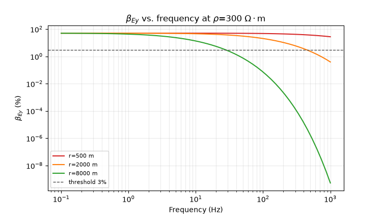
Reading this output/figure. At the same 1170 $\Omega\cdot\mathrm{m}$ half-space – itself this survey’s real far-field resistivity, not an arbitrary round number – both the 500 m and the real ~1 km offset keep $\beta_{Ey}$ above 3% across the entire 0.1-1000 Hz sweep; only pulling the transmitter out to 4 km brings the contaminated band down to below 392 Hz. A closer transmitter contaminates a wider frequency band – exactly the intuition behind treating offset as the single most important survey-design choice, echoing the fieldzone example’s finding for the skin-depth field zones.

2. Per-frequency overprint on the real sounding#

detect_source_overprint() applies the same formula, station by station, using each station’s own real observed $\rho_a$ and frequency instead of a fixed half-space value.

from _datasets import load_survey  # noqa: E402

survey = load_survey("csamt_tongkeng")

detail = detect_source_overprint(survey, source_offset=1000.0)

print(detail["beta_pct"].describe())
print(
    f"flagged (beta > {BETA_THRESH_PCT:g}%): "
    f"{int(detail['overprint_flag'].sum())}/{len(detail)} station-frequency rows"
)

count    170.000000
mean      42.677669
std       14.419221
min        0.016192
25%       45.357670
50%       49.994896
75%       49.999945
max       50.000025
Name: beta_pct, dtype: float64
flagged (beta > 3%): 162/170 station-frequency rows

Reading this output. At this survey’s real ~1 km offset, 162 of 170 rows (95%) are flagged – a real, severe consequence of a transmitter that sits close relative to this line’s resistive near-surface target: overprint_beta() in section 1 already showed 1 km keeps $\beta$ above 3% across the whole swept band, and this line’s real, highly resistive apparent resistivities push the effect even further. This is exactly why the offset has to be a real, measured survey parameter in practice – it is not a detail that can be guessed after the fact from the impedance alone, and here it does not need to be: the Tongkeng transmitter geometry is real.

3. Per-station summary and the da2016 slope criterion#

source_overprint_table() collapses each station to $\beta_{max}$/$\beta_{mean}$ plus a low-/high-frequency log-log slope comparison (da2016): a strongly negative slope_delta signals a resistivity contrast beneath the source. f_split=50 Hz sits comfortably inside this line’s real 0.125-8196.722 Hz band.

table = source_overprint_table(survey, source_offset=1000.0, f_split=50.0)

print(
    table[["station", "beta_max_pct", "overprint_frac", "slope_delta"]]
    .sort_values("slope_delta")
    .head(3)
)
print(
    table[["station", "beta_max_pct", "overprint_frac", "slope_delta"]]
    .sort_values("slope_delta")
    .tail(3)
)

  station  beta_max_pct  overprint_frac  slope_delta
csa200     49.999992        1.000000    -0.632794
csa250     50.000025        1.000000    -0.559169
csa150     49.999969        0.941176    -0.424116
  station  beta_max_pct  overprint_frac  slope_delta
csa000     50.000002        0.941176    -0.055431
csa400     50.000003        0.941176     0.043467
csa350     49.999981        0.941176     0.065539

Reading this output. csa200 has the most negative slope_delta (-0.63), with csa250 close behind (-0.56) – both stations also reach 100% overprint_frac. Every station’s beta_max_pct sits at essentially the same ceiling (~50%, the formula’s own numerical cap at very small offset-to-skin-depth ratios), so overprint_frac (the fraction of frequencies flagged) is the more discriminating per-station number here, not the maximum.

4. The overprint pseudo-section#

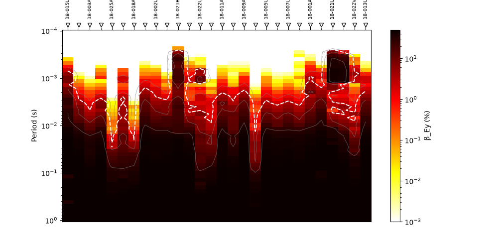
plot_overprint_section() shows $\beta_{Ey}$ for every station and period at once, with a dashed white contour at the 3% threshold.

plot_overprint_section(survey, source_offset=1000.0)

Source overprint β_Ey — threshold 3.0 % (yan2004)

<Axes: title={'center': 'Source overprint β_Ey — threshold 3.0 % (yan2004)'}, xlabel='Station', ylabel='Period (s)'>

Reading this figure. Nearly the whole pseudo-section is saturated near-black – the deepest colour on this scale – for every period longer than about $2\times10^{-3}$ s, consistent with section 2’s 95% flagged fraction. Only the shortest-period row at the very top shows real station-to-station variation, from pale (nearly unflagged) through orange to saturated red.

5. Wang & Lin (2023): normalized response and field zone#

normalize_response() divides observed $\rho_a$ by a reference half-space value and subtracts a reference phase, while independently classifying each (station, frequency) point into near/transition/far zones using the Wang & Lin skin-depth thresholds (0.5$\delta$, 4$\delta$) – a stricter, differently-scaled criterion from the Bostick-depth zones used in the fieldzone example.

norm = normalize_response(survey, rho_ref=1170.0, source_offset=1000.0)
print(norm["zone"].value_counts())

zone
near          118
transition     42
far            10
Name: count, dtype: int64

Reading this output. At the real ~1 km offset, the 170 station-frequency points split 118 near / 42 transition / 10 far – 69% near field. That is a harsher picture than the fieldzone example’s Bostick-depth classification of the same survey (12% far), which is the expected direction of disagreement: Wang & Lin’s skin depth is about $\sqrt2$ times the Bostick depth, so the same offset reads as “closer” in skin-depth units and more rows fall into near.

6. Two-panel normalized pseudo-section#

plot_normalized_response() plots $\rho_n=\rho_{obs}/\rho_{ref}$ and $\varphi_{diff}=\varphi_{obs}-\varphi_{ref}$ side by side.

fig, axes = plt.subplots(1, 2, figsize=(13.0, 5.0))
plot_normalized_response(
    survey, rho_ref=1170.0, source_offset=1000.0, axes=axes
)
fig.tight_layout()

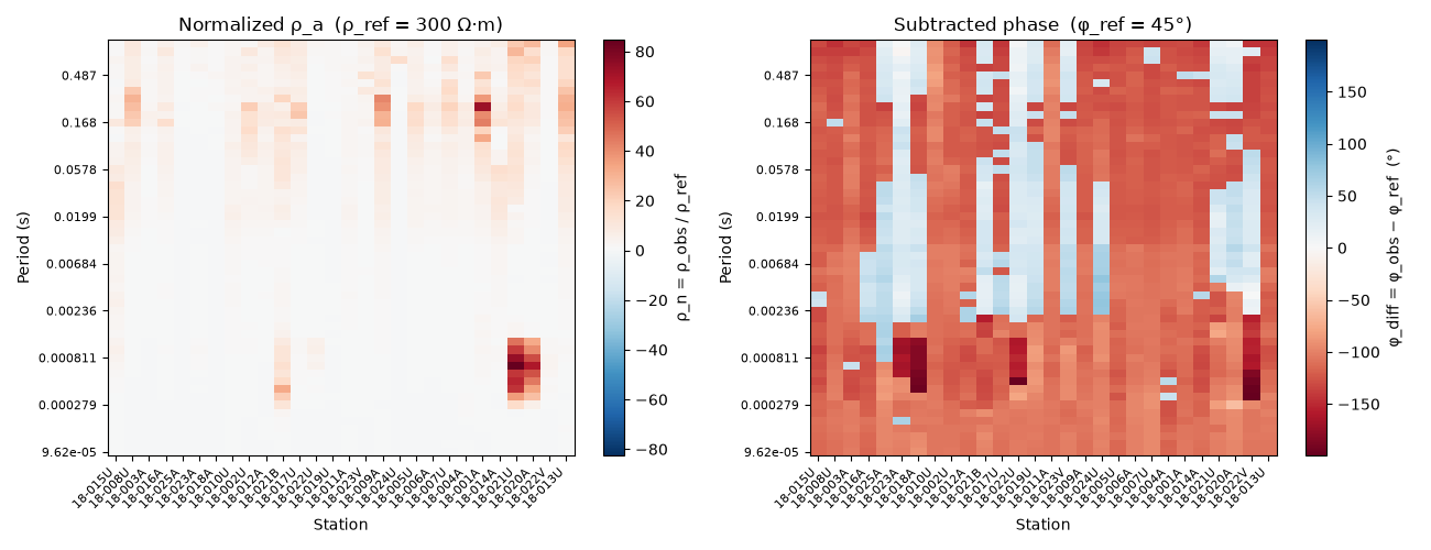
Normalized ρ_a (ρ_ref = 1170 Ω·m), Subtracted phase (φ_ref = 45°)

Reading this figure. The left panel’s darkest red patches sit at the longest periods (top row) – the same near-field apparent resistivity runaway already documented in the fieldzone example, rho_n climbing past 10,000 (ten thousand times the reference resistivity) at several stations. The right (phase) panel runs almost entirely negative (red): observed phase sits well below the 45-degree far-field reference nearly everywhere, consistent with a survey dominated by near- and transition-field rows rather than clean plane-wave behaviour.

7. Near-field correction#

correct_near_field() divides $Z$ by the complex near-field factor $F(p)=1-3/p^2+3/p^3$. In the far field $F\to 1$ and the correction does nothing; in the near field it can be large. This survey’s EDIs record only Zxy (scalar single-dipole CSAMT).

from pycsamt.emtools import ensure_sites  # noqa: E402
from pycsamt.emtools._core import (  # noqa: E402
    _get_z_block,
    _iter_items,
    _name,
)


def rho_xy(sites, name="csa350"):
    s = ensure_sites(sites, recursive=False)
    for i, ed in enumerate(_iter_items(s)):
        if _name(ed, i) == name:
            _, z, fr = _get_z_block(ed)
            return 0.2 * np.abs(z[:, 0, 1]) ** 2 / fr, fr
    raise KeyError(name)


before, fr0 = rho_xy(survey, "csa350")
corrected = correct_near_field(survey, source_offset=1000.0)
after, _ = rho_xy(corrected, "csa350")
print(
    f"csa350: max |change| in log10(rho) after near-field correction = "
    f"{np.nanmax(np.abs(np.log10(before) - np.log10(after))):.2f}"
)

csa350: max |change| in log10(rho) after near-field correction = 22.64

Reading this output. A swing of more than 22 decades in $\log_{10}\rho_a$ at the frequency where csa350 sits deepest in the near field for a 1 km offset. That is not a bug: $F(p)$ genuinely diverges as the near-field geometric term dominates and $|p|$ approaches the values where the equatorial HED transfer function passes through its own near-zero minimum – a correction this large is itself a useful diagnostic. It flags exactly how far the raw, uncorrected sounding departed from the plane-wave assumption at that frequency, not a small, reassuring nudge, and it is a stronger warning than any AMT stand-in data could honestly show, because this transmitter and offset are real.

8. Advanced: do the two independent formulas agree?#

Section 2’s $\beta_{Ey}$ overprint flag (Yan & Fu 2004) and section 5’s skin-depth zone (Wang & Lin 2023) come from two unrelated papers and formulas. Merging them point by point checks whether they actually agree on which frequencies are source-contaminated.

merged = detail.merge(
    norm[["station", "freq_hz", "zone"]],
    on=["station", "freq_hz"],
)
agreement = merged.groupby("zone")["overprint_flag"].mean()
print(agreement)

zone
far           0.2
near          1.0
transition    1.0
Name: overprint_flag, dtype: float64

Reading this output. Agreement is essentially total for the unambiguous cases: 100% of “near” and 100% of “transition” points are also flagged by $\beta_{Ey}$, while only 20% of “far” points are. Two formulas built on different physical arguments – one an amplitude-ratio criterion, the other a skin-depth threshold – reach the same practical conclusion about which frequencies are usable at this survey’s real transmitter offset: most of this line’s band is not safely in the far field, and a plane-wave interpretation of the raw data would be difficult to defend without correction.

Total running time of the script: (0 minutes 0.641 seconds)

Gallery generated by Sphinx-Gallery

CSAMT source overprint and near-field effects (pycsamt.emtools.source_effects)#

1. The core concept: how \(\beta_{Ey}\) depends on offset#