
11.8. Geoelectric Strike#
Geoelectric strike is the preferred 2-D structural direction inferred from electromagnetic data. It is one of the checks you make before rotating impedances, preparing 2-D inversion inputs, or interpreting TE mode and TM mode responses. In pyCSAMT, the strike tools estimate the direction from impedance rotation, phase tensor azimuth, or a consensus of both, then visualize the result as tables, profiles, ribbons, map-sticks, and rose diagrams.
Strike angles are axial. A strike of 0 degrees and a strike of
180 degrees are the same geological direction. For that reason,
pyCSAMT reports station-level strike in the compact [-90, 90] range
for estimator tables, while rose diagrams fold angles into 0 to
180 and mirror the histogram around the full polar circle.
The wrapping used throughout the strike tools is
Here \(\theta\) is any strike angle in degrees. This convention keeps equivalent axes, such as \(-80^\circ\) and \(100^\circ\), on the same branch before station medians, differences, or plots are computed.
Use this page when you need to answer concrete processing questions:
Question |
Main tools |
Output |
|---|---|---|
What strike does each station prefer? |
|
One row per station with angle, stability, period band, and sample count. |
Does strike change with period? |
|
One angle per station and frequency, plus a ribbon image. |
What strike should I rotate to? |
|
A corrected |
How do lines or bands compare? |
|
Axial rose diagrams with weighted mean directions. |
Is the strike spatially coherent? |
|
Along-line and geographic views. |
How does Z strike compare with phase tensor and tipper direction? |
|
Strike and PT azimuth rose diagram, plus tipper rose when present. |
The examples use the public two-level import style:
from pycsamt.emtools import ....
11.8.1. Load Data#
Load the survey with ensure_sites first. This gives every strike
function the same clean input and avoids repeating EDI parsing options in
every call.
>>> from pathlib import Path
>>> import numpy as np
>>> from pycsamt.emtools import ensure_sites
>>> edi_dir = Path("data/AMT/WILLY_DATA/L18PLT")
>>> sites = ensure_sites(edi_dir, recursive=True, verbose=0)
For map and profile plots, coordinates matter. plot_strike_profile
can order stations by "lon", "lat", "name", or "auto".
Choose the ordering that matches the survey line, not merely the default.
For a north-south line, sort_by="lat" is often the clearer choice.
For an east-west line, sort_by="lon" is usually better.
11.8.2. Station-Level Estimators#
pyCSAMT provides three station-level strike estimators. They all return
a pandas.DataFrame with the same practical columns:
Column |
Meaning |
|---|---|
|
Station identifier. |
|
Estimated strike angle in degrees, wrapped into |
|
Interquartile range of the frequency-level estimates used to summarize the station. Smaller values mean a more stable strike. |
|
Period-band limits in seconds used by the estimate. |
|
Number of frequency samples used. |
The impedance sweep rotates each tensor through a grid of trial angles and chooses the angle that optimizes a metric. For a trial angle \(\alpha\), the impedance tensor is rotated as
The default sweep metric (metric="diag_ratio") compares the diagonal
and off-diagonal energy after rotation,
The frequency-level strike is the trial angle that minimizes
\(S(\alpha, f)\). The station-level value reported as ang is
the axial median of those frequency-level angles inside the selected
period band, after unwrapping jumps across the \(\pm 90^\circ\)
boundary. The reported iqr is the interquartile range of the same
unwrapped angle population.
>>> from pycsamt.emtools import estimate_strike_sweep
>>> sweep = estimate_strike_sweep(
...     sites,
...     angles=np.arange(-90.0, 91.0, 1.0),
...     metric="diag_ratio",
...     band=(0.001, 10.0),
... )
>>> print(sweep[["station", "ang", "iqr", "n"]])
    station   ang    iqr   n
0   18-001A  34.0  175.5  39
1   18-002U  32.0  248.5  39
2   18-003A -21.0  305.5  39
3   18-004A -67.0  199.0  39
4   18-005U -36.0  181.0  39
5   18-006A -33.0  185.5  39
6   18-007U -41.0  165.0  39
7   18-008U -34.0  169.5  39
8   18-009A -75.0  177.0  39
9   18-010U -17.0   35.5  39
10  18-011A  76.0  185.0  39
11  18-012A -49.0   49.0  39
12  18-013U -38.0   49.5  39
13  18-014A -47.0  165.5  39
14  18-015U -13.0   85.0  39
15  18-016A  -8.0   84.0  39
16  18-017U -42.0   77.5  39
17  18-018A -14.0   55.0  39
18  18-019U -22.0  322.5  39
19  18-020A -37.0   96.5  39
20  18-021U -29.0   24.5  39
21  18-021B -25.0  104.0  39
22  18-022U -19.0   56.0  39
23  18-022V -53.0  146.5  39
24  18-023A -23.0   82.0  39
25  18-023V -46.0   45.0  39
26  18-024U -75.0   44.0  39
27  18-025A -66.0  319.0  39
Most iqr values here sit between 50 and 250 degrees, which is
large. diag_ratio searches for the rotation that minimizes diagonal
energy relative to off-diagonal energy – a useful impedance-based strike
diagnostic, but one that is sensitive to noise, 3-D effects, and weak
diagonal/off-diagonal contrast at any single frequency. Do not treat a
single-frequency sweep angle as reliable; the station-level median over a
band is what makes the estimate usable.
The phase-tensor estimator summarizes the phase tensor theta angle.
It is often more stable than a raw impedance sweep because the
phase tensor is less affected by static shift amplitude
distortion. Writing the complex impedance as
\(\mathbf{Z}=\mathbf{X}+i\mathbf{Y}\), the phase tensor is
Static shift changes real apparent-resistivity amplitudes, but it does
not multiply \(\mathbf{X}\) and \(\mathbf{Y}\) by different
factors. The phase tensor therefore preserves directional phase
information that is often cleaner than the amplitude-sensitive sweep.
estimate_strike_phase_tensor takes the tensor azimuth
\(\theta_{\Phi}(f)\) at each frequency and reports its robust axial
median over the chosen period band.
>>> from pycsamt.emtools import estimate_strike_phase_tensor
>>> pt = estimate_strike_phase_tensor(
...     sites,
...     band=(0.001, 10.0),
...     robust=True,
... )
>>> print(pt[["station", "ang", "iqr", "n"]])
    station        ang         iqr   n
0   18-001A -44.641194   33.507488  39
1   18-002U -43.757578   13.310763  39
2   18-003A -37.153258   12.725693  39
3   18-004A -40.889492   17.540830  39
4   18-005U -42.404158   14.929706  39
5   18-006A -42.558905   26.757145  39
6   18-007U -45.967488   19.748005  39
7   18-008U -45.374795   33.130660  39
8   18-009A -40.484848   13.871500  39
9   18-010U -43.432226   19.080351  39
10  18-011A -40.391078   18.967773  39
11  18-012A -39.419545   26.067880  39
12  18-013U -41.742580   31.608457  39
13  18-014A -22.821394   72.754984  39
14  18-015U -33.387647  169.387460  39
15  18-016A -20.658294   24.764908  39
16  18-017U -26.561809   27.729096  39
17  18-018A -33.728193   13.362541  39
18  18-019U -31.821680   25.741787  39
19  18-020A -30.044215    6.472585  39
20  18-021B -21.755190   97.461766  39
21  18-021U -28.191808    6.079438  39
22  18-022U -28.484481  152.548514  39
23  18-022V -22.375149   18.359603  39
24  18-023A -41.324136  155.368896  39
25  18-023V -50.745390   40.183828  39
26  18-024U -51.114376   11.877314  39
27  18-025A -40.069989   24.228480  39
The phase-tensor table is the cleanest of the three: most iqr values
sit well under 40 degrees and the ang column clusters tightly
around -40 degrees. A handful of stations (18-014A, 18-015U,
18-022U, 18-023A) break that pattern with much larger iqr
values; treat those as unstable regardless of which estimator produced
them.
The consensus estimator blends the sweep and phase-tensor estimates. Use it when neither method should dominate the processing decision. Before blending, pyCSAMT places both angles on the same axial branch. A two-estimator consensus can be read as
where \(\tilde{\theta}_s\) is the unwrapped sweep estimate, \(\tilde{\theta}_\Phi\) is the unwrapped phase-tensor estimate, and \(w_s\) and \(w_\Phi\) are the sweep and phase-tensor weights. Use weights that sum to one when you want the consensus to remain a direct weighted average.
>>> from pycsamt.emtools import estimate_strike_consensus
>>> consensus = estimate_strike_consensus(
...     sites,
...     band=(0.001, 10.0),
...     w_sweep=0.4,
...     w_pt=0.6,
...     metric="diag_ratio",
... )
>>> print(consensus[["station", "ang", "iqr", "n"]])
    station        ang         iqr   n
0   18-001A -13.184716  104.503744  78
1   18-002U -13.454547  130.905381  78
2   18-003A -30.691955  159.112846  78
3   18-004A -51.333695  108.270415  78
4   18-005U -39.842495   97.964853  78
5   18-006A -38.735343  106.128573  78
6   18-007U -43.980493   92.374002  78
7   18-008U -40.824877  101.315330  78
8   18-009A -54.290909   95.435750  78
9   18-010U -32.859336   27.290176  78
10  18-011A   6.165353  101.983886  78
11  18-012A -43.251727   37.533940  78
12  18-013U -40.245548   40.554228  78
13  18-014A -32.492836  119.127492  78
14  18-015U -25.232588  127.193730  78
15  18-016A -15.594976   54.382454  78
16  18-017U -32.737085   52.614548  78
17  18-018A -25.836916   34.181271  78
18  18-019U -27.893008  174.120894  78
19  18-020A -32.826529   51.486293  78
20  18-021U -28.515085   15.289719  78
21  18-021B -23.053114  100.730883  78
22  18-022U -24.690689  104.274257  78
23  18-022V -34.625089   82.429802  78
24  18-023A -33.994482  118.684448  78
25  18-023V -48.847234   42.591914  78
26  18-024U -60.668626   27.938657  78
27  18-025A -50.441993  171.614240  78
n roughly doubles in the consensus table because it is the sum of
sweep and phase-tensor sample counts, not a separate independent count.
For all three tables, treat iqr as a stability warning. Station
18-011A illustrates why: the sweep angle is 76.0 degrees, the
phase-tensor angle is -40.4 degrees, and the consensus lands at
6.2 degrees with a high iqr – the two estimators disagree enough
that the blended number does not represent a confident single strike at
that station.
11.8.3. Compare Axial Angles Correctly#
Do not compare strike estimates with ordinary subtraction unless you
first account for the 180 degree ambiguity. The axial difference
between 89 and -89 degrees is 2 degrees, not 178 degrees.
For two angles \(\theta_1\) and \(\theta_2\), use
>>> merged = sweep.merge(
...     pt,
...     on="station",
...     suffixes=("_sweep", "_pt"),
... )
>>> axial_diff = (
...     (merged["ang_sweep"] - merged["ang_pt"] + 90.0) % 180.0
... ) - 90.0
>>> merged["abs_axial_diff"] = axial_diff.abs()
>>> print(
...     merged[
...         ["station", "ang_sweep", "ang_pt", "abs_axial_diff"]
...     ].sort_values("abs_axial_diff", ascending=False)
... )
    station  ang_sweep     ang_pt  abs_axial_diff
0   18-001A       34.0 -44.641194       78.641194
1   18-002U       32.0 -43.757578       75.757578
10  18-011A       76.0 -40.391078       63.608922
8   18-009A      -75.0 -40.484848       34.515152
23  18-022V      -53.0 -22.375149       30.624851
9   18-010U      -17.0 -43.432226       26.432226
3   18-004A      -67.0 -40.889492       26.110508
27  18-025A      -66.0 -40.069989       25.930011
13  18-014A      -47.0 -22.821394       24.178606
26  18-024U      -75.0 -51.114376       23.885624
14  18-015U      -13.0 -33.387647       20.387647
17  18-018A      -14.0 -33.728193       19.728193
24  18-023A      -23.0 -41.324136       18.324136
2   18-003A      -21.0 -37.153258       16.153258
16  18-017U      -42.0 -26.561809       15.438191
15  18-016A       -8.0 -20.658294       12.658294
7   18-008U      -34.0 -45.374795       11.374795
18  18-019U      -22.0 -31.821680        9.821680
11  18-012A      -49.0 -39.419545        9.580455
5   18-006A      -33.0 -42.558905        9.558905
22  18-022U      -19.0 -28.484481        9.484481
19  18-020A      -37.0 -30.044215        6.955785
4   18-005U      -36.0 -42.404158        6.404158
6   18-007U      -41.0 -45.967488        4.967488
25  18-023V      -46.0 -50.745390        4.745390
12  18-013U      -38.0 -41.742580        3.742580
21  18-021B      -25.0 -21.755190        3.244810
20  18-021U      -29.0 -28.191808        0.808192
Roughly a third of the survey shows better than 10 degrees of
agreement between the two estimators; the top of the table is dominated
by the same high-iqr stations already flagged above (18-001A,
18-002U, 18-011A). Use this comparison pattern whenever you
compare sweep, phase tensor, consensus, tipper azimuth, or externally
interpreted structural trends. A naive Pearson correlation of raw angles
can be misleading because it treats the wrap boundary as a real
discontinuity.
11.8.4. Choose A Period Band#
The band argument is a period band in seconds. It is available on
the station-level estimators and on the high-level plots that summarize
station-level strike. Use it to separate shallow, high-frequency
behavior from deeper, long-period behavior.
>>> short_period = estimate_strike_consensus(
...     sites,
...     band=(0.001, 0.1),
... )
>>> long_period = estimate_strike_consensus(
...     sites,
...     band=(0.1, 10.0),
... )
>>> band_compare = short_period[["station", "ang", "iqr"]].merge(
...     long_period[["station", "ang", "iqr"]],
...     on="station",
...     suffixes=("_short", "_long"),
... )
>>> band_compare["band_axial_diff"] = (
...     (band_compare["ang_short"] - band_compare["ang_long"] + 90.0)
...     % 180.0
... ) - 90.0
>>> print(band_compare)
    station  ang_short   iqr_short   ang_long    iqr_long  band_axial_diff
0   18-001A -54.506201   41.369421 -63.900455  123.466880         9.394254
1   18-002U -48.985879  160.057160 -36.157439   19.623319       -12.828440
2   18-003A  19.394690   78.014960 -22.303922   91.734047        41.698612
3   18-004A  13.847161   90.942272 -27.625934   87.492859        41.473095
4   18-005U   6.699252  139.105342 -32.804464    8.183583        39.503716
5   18-006A -45.672788   25.902400 -27.695474   15.377996       -17.977315
6   18-007U -43.969709   97.304264 -40.122137    5.186640        -3.847572
7   18-008U  -9.158404  101.878737 -41.169270   27.580778        32.010866
8   18-009A -54.850045   44.971449 -25.514648   51.649186       -29.335397
9   18-010U -38.081566   29.303524 -22.194658   95.009109       -15.886908
10  18-011A -27.725972   74.750686 -23.482145    6.419555        -4.243828
11  18-012A -52.101381   30.124857 -24.691455   11.576741       -27.409926
12  18-013U -45.827104   71.741797 -30.024716   12.679180       -15.802388
13  18-014A -29.010735   47.579291  -1.990831   87.090185       -27.019904
14  18-015U -22.291812   94.794970   1.541876  138.925951       -23.833688
15  18-016A -44.272043   60.760395 -15.286250   92.857554       -28.985794
16  18-017U -60.409554   37.127807  31.430982   92.784065        88.159465
17  18-018A -23.871328   47.793334 -36.763786   97.172580        12.892458
18  18-019U  26.599036   81.719385 -34.186076   31.783625        60.785112
19  18-020A -60.182514   85.406263 -32.313086    3.341403       -27.869429
20  18-021U -27.000027   18.589938 -29.192501    3.856444         2.192474
21  18-021B -17.977499   83.255421 -22.009438   56.404952         4.031939
22  18-022U  -5.488390  103.595335 -24.809677   54.724645        19.321287
23  18-022V  -0.989376   80.416924 -30.666820    4.212487        29.677445
24  18-023A -32.013201  115.048817 -16.838399   49.906991       -15.174802
25  18-023V -49.434564   52.035662 -61.711376   86.588207        12.276812
26  18-024U -68.098458   50.928656 -45.399175   33.879698       -22.699283
27  18-025A -15.407326  101.090032 -39.573699   66.987043        24.166372
Stations 18-017U and 18-019U swing by more than 60 degrees
between the short- and long-period bands, and both bands still carry
large iqr values at most stations. If short- and long-period strikes
disagree strongly, do not force a single rotation across the entire
band. Review dimensionality, static shift, near-surface diagnostics, and
the inversion band before choosing a processing strike.
11.8.5. Rotate Data Onto Strike#
rotate_to_strike estimates one strike angle per station and rotates
that station’s impedance tensor. Keep the original and rotated data
separate until you have checked the result. For station \(s\), the
rotation applied to every frequency sample is
where \(\theta_s\) is the station-level strike selected by the requested method. In a 2-D interpretation this tries to place the dominant response into the off-diagonal modes, but the formula is only a coordinate rotation; it does not remove 3-D induction or bad data.
>>> from pycsamt.emtools import rotate_to_strike
>>> rotated = rotate_to_strike(
...     sites,
...     method="consensus",
...     band=(0.001, 10.0),
...     metric="diag_ratio",
...     inplace=False,
... )
>>> before = estimate_strike_consensus(
...     sites,
...     band=(0.001, 10.0),
... )
>>> after = estimate_strike_consensus(
...     rotated,
...     band=(0.001, 10.0),
... )
>>> print("before mean abs strike:", before["ang"].abs().mean())
before mean abs strike: 33.75926323036427
>>> print("after mean abs strike:", after["ang"].abs().mean())
after mean abs strike: 23.699459229145212
Re-estimating strike on the rotated survey pulls the mean absolute angle
from about 34 degrees down to about 24 degrees, which is the
expected direction of change: rotation moves the dominant axis closer to
0/90 in the rotated frame, it does not force it there exactly.
Valid method names are "consensus", "sweep", and "pt". Use
inplace=False while building a workflow; it returns a rotated copy
and keeps the unrotated survey available for before/after checks.
Rotation does not make a survey 2-D by itself. If the selected band has
high skew, unstable strike, or strong station-to-station disagreement,
the rotated tensors may still be poor 2-D inversion input.
11.8.6. Per-Frequency Strike Curve#
strike_curve_sweep keeps the frequency dimension instead of reducing
each station to one number. It is useful for finding unstable bands or
stations whose strike flips with period.
>>> from pycsamt.emtools import strike_curve_sweep
>>> curve = strike_curve_sweep(
...     sites,
...     angles=np.arange(-90.0, 91.0, 1.0),
...     metric="diag_ratio",
...     smooth=5,
... )
>>> print(curve.head())
   station     freq    period   ang
0  18-001A  10400.0  0.000096  59.0
1  18-001A   8707.0  0.000115 -78.2
2  18-001A   7289.0  0.000137 -36.2
3  18-001A   6102.0  0.000164  -2.2
4  18-001A   5108.0  0.000196  -3.2
>>> print(curve.groupby("station")["ang"].agg(["median", "std", "count"]))
         median        std  count
station
18-001A   -27.4  52.458417     53
18-002U   -45.8  60.834128     53
18-003A   -22.4  46.238784     53
18-004A   -21.6  50.020511     53
18-005U   -18.6  43.659775     53
18-006A   -37.8  34.259013     53
18-007U   -43.8  38.061708     53
18-008U   -47.4  45.431997     53
18-009A   -16.0  47.725733     53
18-010U   -18.6  44.842346     53
18-011A    -9.8  47.598151     53
18-012A   -40.8  39.072262     53
18-013U   -38.0  48.110960     53
18-014A   -24.2  32.911592     53
18-015U   -16.4  49.769125     53
18-016A   -46.2  33.376512     53
18-017U   -66.0  41.357284     53
18-018A   -19.6  37.349080     53
18-019U   -21.8  50.727413     53
18-020A   -31.8  31.427665     53
18-021B   -23.2  38.380236     53
18-021U   -33.2  36.604952     53
18-022U   -38.8  32.873812     53
18-022V   -37.2  38.037783     53
18-023A   -28.6  48.879846     53
18-023V   -40.6  33.763535     53
18-024U   -36.2  56.412705     53
18-025A   -29.0  54.837346     53
The table columns are station, freq, and ang. smooth
applies a moving average to the frequency-level sweep angles before they
are wrapped back into the axial range. Increase it only when you want a
smoother visual trend; do not use smoothing to hide genuine strike
changes. Every std in the summary above exceeds 30 degrees –
consistent with the noisy, unstable single-frequency sweep angles seen
earlier – which is exactly why the station-level estimators reduce the
curve to a robust median rather than reporting a single frequency’s
value.
The smoothing is applied to an unwrapped axial sequence, so a transition near \(90^\circ\) is treated as a continuation of the same axis rather than a jump across the plot. With an odd window length \(m\), the displayed trend is approximately
where \(\tilde{\theta}_k\) are the locally unwrapped frequency-level sweep angles.
11.8.7. Ribbon Plot#
plot_strike_ribbon converts the per-frequency strike curve to a
station-by-period image. Hue encodes strike angle. Saturation encodes
local stability: desaturated colors indicate high local variance. This
makes the ribbon more than a color table – a saturated, coherent stripe
means nearby period samples agree on the same axial direction, while a
pale or mottled interval means the local angular variance is high, so a
single strike from that interval should be treated cautiously.
>>> import matplotlib.pyplot as plt
>>> from pycsamt.emtools import plot_strike_ribbon
>>> ax = plot_strike_ribbon(
...     sites,
...     method="sweep",
...     win=5,
...     show_colorbar=True,
... )
>>> ax.figure.savefig("strike_ribbon.png", dpi=200, bbox_inches="tight")
>>> plt.close(ax.figure)
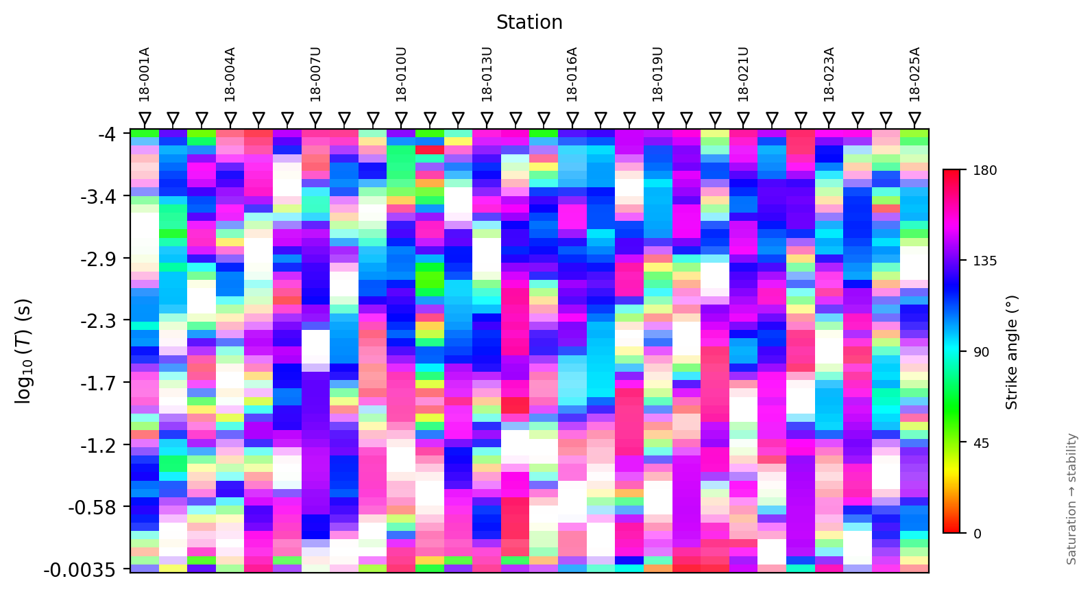
The ribbon confirms the picture from the curve table: colors change
station to station and period to period across most of the survey,
matching the large std values reported above. Use the ribbon before
selecting a single strike for a broad period band. If it changes color
systematically from short period to long period, the survey may need
band-specific interpretation.
11.8.8. Rose Diagrams#
plot_strike_rose draws axial strike histograms styled with the
"pycsamt" RoseStyle preset by default: gradient-colored bars, a
bold outer ring, a crimson mean-direction spike, a dashed secondary-axis
line, and an annotation box reporting the mean angle and station count.
It mirrors the 0 to 180 degree histogram around the full circle,
so both halves of the polar plot represent the same set of axes.
When inverse-IQR weighting is requested, stations with stable frequency behavior carry more weight:
The rose mean is computed as an axial mean, not an ordinary circular mean. Internally this is equivalent to doubling the angles, averaging the unit vectors, and halving the result:
>>> from pycsamt.emtools import plot_strike_rose
>>> fig = plot_strike_rose(
...     sites,
...     method="consensus",
...     band=(0.001, 10.0),
...     bins=36,
...     weight="inv_iqr",
...     suptitle="Consensus geoelectric strike",
... )
>>> fig.savefig("strike_rose_consensus.png", dpi=200, bbox_inches="tight")
>>> plt.close(fig)
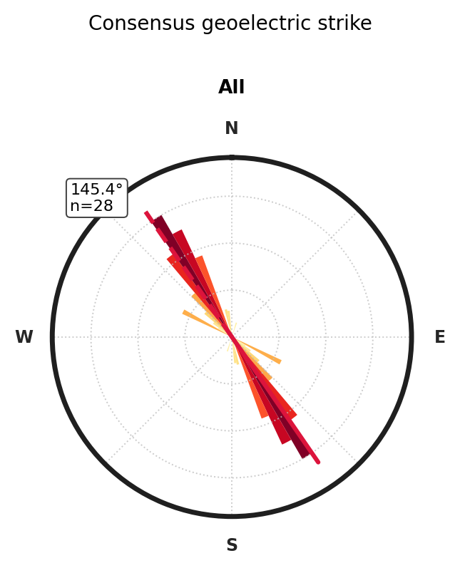
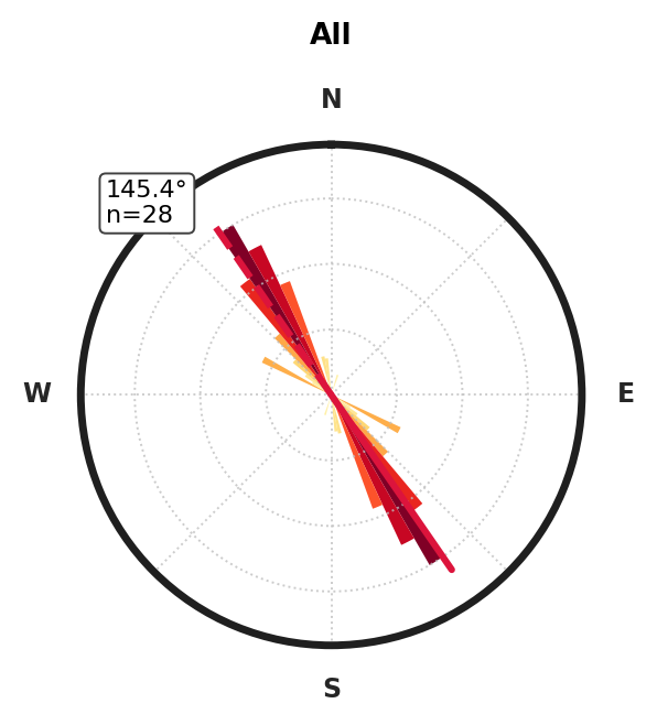
The weighted mean lands at 145.4 degrees (equivalently -34.6
degrees on the compact axial scale), which sits close to the
phase-tensor cluster seen in the station table. weight="inv_iqr"
down-weights stations whose strike varies strongly with frequency; use
weight="uniform" when every station should contribute equally.
When groups is omitted, pyCSAMT attempts to group stations by a
profile-like station-name prefix. This works for names such as
E1S01 because the inferred group is E1. For station names that
do not encode the line this way, pass an explicit mapping. L18PLT and
L22PLT are two separate AMT lines from the same survey, so comparing
them checks whether the regional strike is consistent along strike or
only a property of one profile.
>>> from pathlib import Path
>>> line18 = sorted(Path("data/AMT/WILLY_DATA/L18PLT").glob("*.edi"))
>>> line22 = sorted(Path("data/AMT/WILLY_DATA/L22PLT").glob("*.edi"))
>>> groups = {
...     "L18PLT": [path.stem for path in line18],
...     "L22PLT": [path.stem for path in line22],
... }
>>> fig = plot_strike_rose(
...     line18 + line22,
...     groups=groups,
...     method="consensus",
...     bins=36,
...     n_cols=2,
...     suptitle="Strike by profile line",
... )
>>> fig.savefig("strike_rose_profiles.png", dpi=200, bbox_inches="tight")
>>> plt.close(fig)
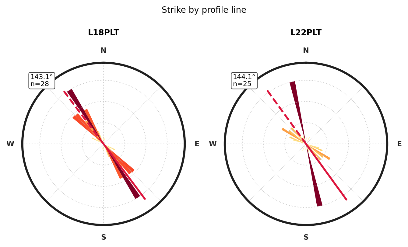
L18PLT and L22PLT agree to within one degree (143.1 versus 144.1
degrees), which is strong evidence that the estimated direction reflects
a regional structural trend rather than an artifact of one particular
line’s geometry or noise.
plot_strike_rose_by_line is a simpler line-comparison helper. It
draws each group with plain degree ticks rather than the full compass
styling above, and requires at least two stations per group; if
automatic grouping produces only singleton groups, pass the explicit
groups dictionary yourself.
>>> from pycsamt.emtools import plot_strike_rose_by_line
>>> fig = plot_strike_rose_by_line(
...     line18 + line22,
...     groups=groups,
...     method="consensus",
...     band=(0.001, 10.0),
...     weight="inv_iqr",
... )
>>> fig.savefig("strike_rose_by_line.png", dpi=200, bbox_inches="tight")
>>> plt.close(fig)
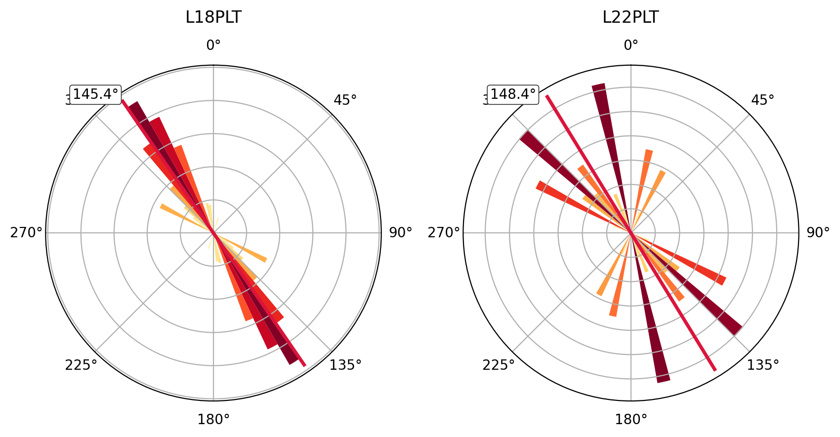
Both lines again cluster tightly around the same 145-ish degree
direction (145.4 and 148.4 degrees here), reinforcing the
profile-comparison result above with a lighter, quick-look plot.
11.8.9. Frequency-Band Roses#
Use bar_style="bands" when you want one rose diagram to show several
period bands. Each band contributes its own stacked histogram.
>>> fig = plot_strike_rose(
...     sites,
...     method="consensus",
...     bar_style="bands",
...     freq_bands=[
...         (0.001, 0.01),
...         (0.01, 0.1),
...         (0.1, 10.0),
...     ],
...     band_labels=[
...         "very short period",
...         "short period",
...         "long period",
...     ],
...     suptitle="Strike by period band",
... )
>>> fig.savefig("strike_rose_bands.png", dpi=200, bbox_inches="tight")
>>> plt.close(fig)
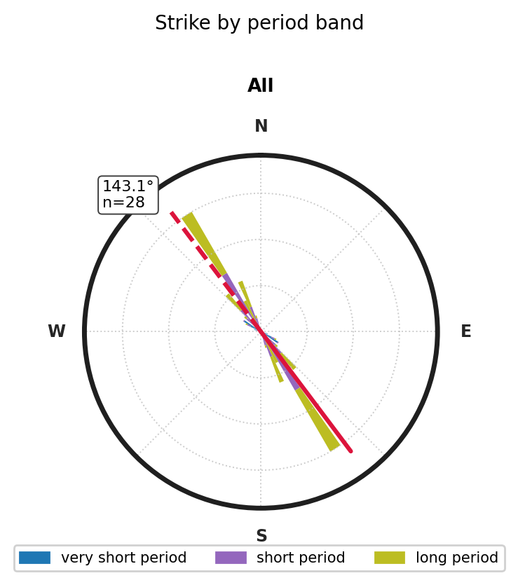
The long-period band dominates the count and carries most of the 145
degree signal, while the very-short-period band is thin – fewer stations
have a stable strike at the shortest periods, which matches the noisy
ribbon plot above. If the bands stack around clearly different mean
directions, report the band-specific behavior instead of collapsing it
to one survey-wide number.
11.8.10. Profile And Map-Stick Views#
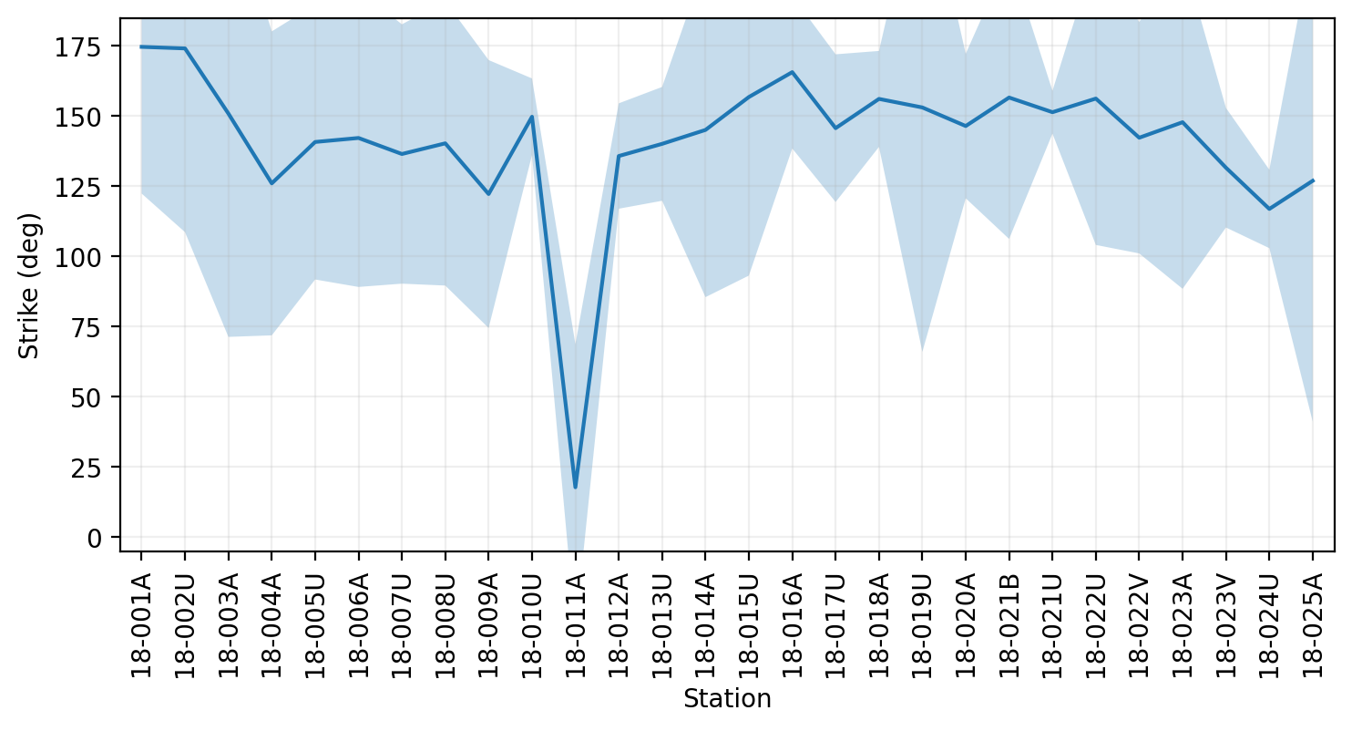
plot_strike_profile shows strike angle along station order with an
IQR ribbon. It is the best quick check for station-to-station
coherence.
>>> from pycsamt.emtools import plot_strike_profile
>>> ax = plot_strike_profile(
...     sites,
...     method="consensus",
...     band=(0.001, 10.0),
...     sort_by="lat",
... )
>>> ax.figure.savefig("strike_profile.png", dpi=200, bbox_inches="tight")
>>> plt.close(ax.figure)
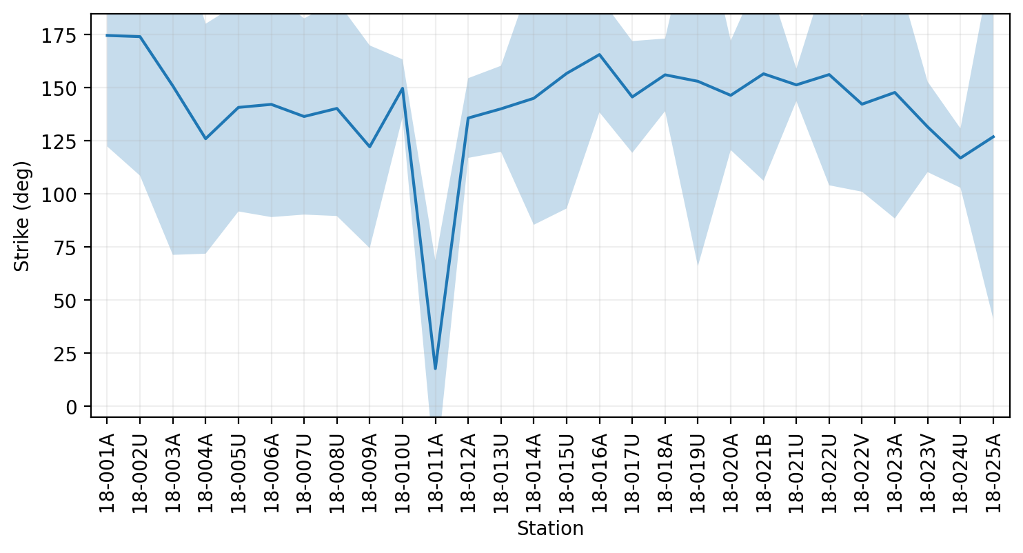
Most of the profile holds between about 120 and 175 degrees with
a moderate IQR ribbon, consistent with a broadly coherent 2-D line.
Station 18-011A is the clear exception – it drops to about 20
degrees, matching the same station flagged earlier for large
sweep/phase-tensor disagreement. A coherent 2-D line should not show
random jumps from station to station unless there is a real geological
or data-quality reason, and this is exactly the kind of single-station
outlier that a survey-wide statistic like the rose mean would hide.
plot_strike_mapsticks draws a short line segment at each station
coordinate, oriented along the estimated strike. It is useful for
checking whether nearby stations point in a consistent direction.
>>> from pycsamt.emtools import plot_strike_mapsticks
>>> ax = plot_strike_mapsticks(
...     sites,
...     method="consensus",
...     band=(0.001, 10.0),
...     len_deg=0.02,
... )
>>> lats = [site.coords[0] for site in sites if site.coords]
>>> lons = [site.coords[1] for site in sites if site.coords]
>>> lon_pad = (max(lons) - min(lons)) * 0.15
>>> lat_pad = (max(lats) - min(lats)) * 0.15
>>> _ = ax.set_xlim(min(lons) - lon_pad, max(lons) + lon_pad)
>>> _ = ax.set_ylim(min(lats) - lat_pad, max(lats) + lat_pad)
>>> _ = ax.set_aspect("auto", adjustable="box")
>>> ax.ticklabel_format(axis="x", style="plain", useOffset=False)
>>> ax.figure.savefig("strike_mapsticks.png", dpi=200, bbox_inches="tight")
>>> plt.close(ax.figure)
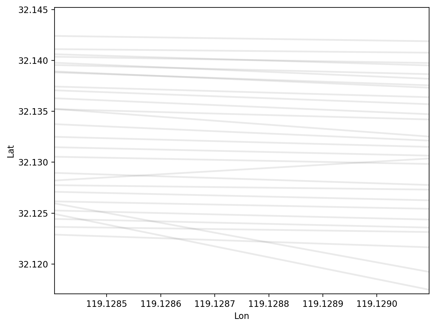
Neighboring sticks tilt in visibly consistent directions along most of
the line, which is the same coherence the profile plot showed, now in
map view. The len_deg value is a display length in coordinate
degrees, not a geological length; adjust it for readability when the
survey extent is very small or very large.
11.8.11. Combined Strike Analysis#
plot_strike_analysis draws a rose figure of impedance strike and
phase-tensor azimuth, adding a third tipper strike panel only
when sites actually carries vertical magnetic transfer functions
somewhere in the survey. A survey with no tipper channel at all gets a
two-panel figure rather than a third panel that would only ever read “no
data”. L18PLT is AMT, with no vertical-field channel, so it is a
two-panel example.
>>> from pycsamt.emtools import plot_strike_analysis
>>> fig = plot_strike_analysis(
...     sites,
...     method="consensus",
...     band=(0.001, 10.0),
...     bins=36,
...     suptitle="Strike and phase-tensor azimuth -- L18PLT (AMT, no tipper)",
... )
>>> fig.savefig("strike_analysis_l18plt.png", dpi=200, bbox_inches="tight")
>>> plt.close(fig)
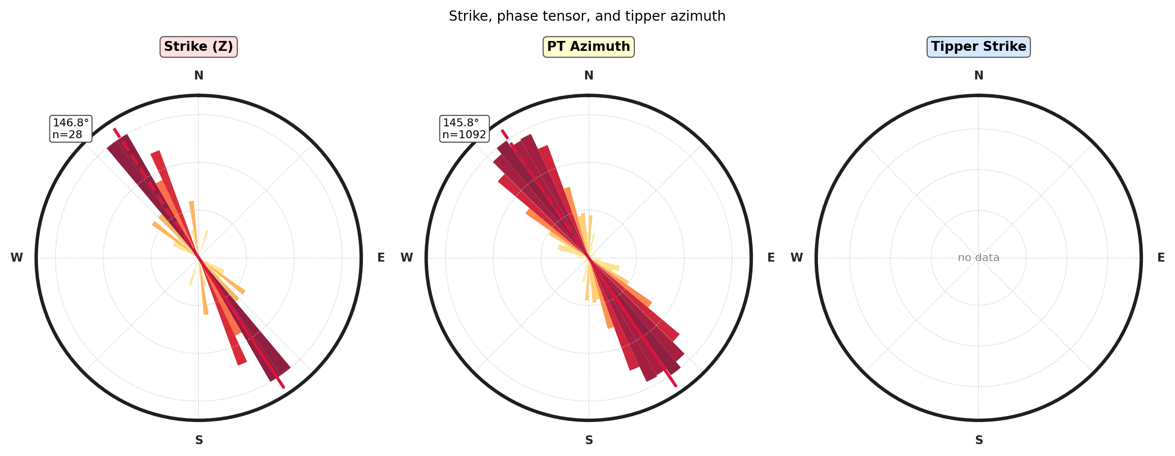
Strike (Z) reports 146.8 degrees from 28 station-level estimates,
and PT Azimuth reports 145.8 degrees from 1092 individual
frequency samples (28 stations times up to 39 frequencies each).
The two panel counts are not meant to match: the Strike (Z) panel
summarizes one robust angle per station, while PT Azimuth plots every
frequency-level phase-tensor sample directly. The near-identical mean
direction from two very differently sized populations is itself a good
consistency check.
To see the third panel with a real survey, switch to data/MT/kap03lmt_edis:
a 26-station real MT line from the SAMTEX archive that, unlike the AMT
lines above, carries genuine vertical-field (tipper) data at every
station.
>>> kap = ensure_sites("data/MT/kap03lmt_edis", recursive=True, verbose=0)
>>> fig = plot_strike_analysis(
...     kap,
...     method="consensus",
...     band=(1.0, 1000.0),
...     bins=36,
...     suptitle="Strike, phase-tensor azimuth, and tipper strike -- KAP03 (MT, real tipper)",
... )
>>> fig.savefig("strike_analysis_kap03.png", dpi=200, bbox_inches="tight")
>>> plt.close(fig)
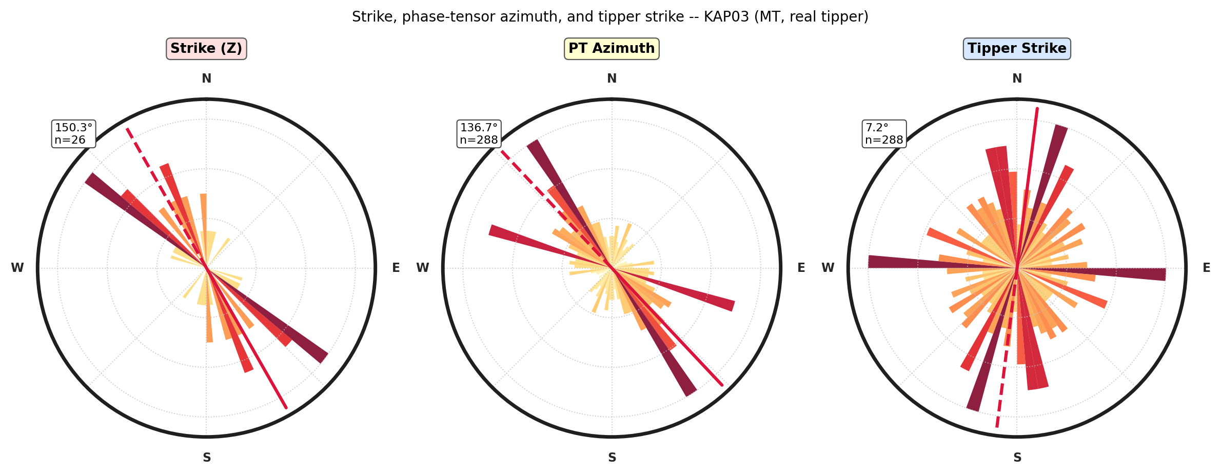
For tipper vectors, pyCSAMT uses the real induction vector direction
where \(T_{zx}\) and \(T_{zy}\) are the horizontal magnetic-field
transfer functions into the vertical magnetic component. Here, Strike
(Z) and PT Azimuth still agree closely (150.3 and 136.7 degrees),
but Tipper Strike points in a very different direction (7.2 degrees,
essentially north-south) and is visibly more scattered around the polar
plot than the other two panels. KAP03 is a long-period, widely spaced
MT line (roughly 60 km station spacing) sensitive to much deeper
structure than the impedance and phase-tensor strike, so this is not a
contradiction to resolve by picking a “correct” panel – it is exactly
the kind of independent directional evidence this figure exists to
surface. Compare tipper azimuth with impedance and phase-tensor strike
as a diagnostic, not as a guaranteed rotation angle: investigate regional
3-D structure, coast effects, cultural noise, or sign convention before
choosing a rotation based on it alone.
11.8.12. Recommended Workflow#
A robust strike workflow keeps estimation, comparison, visualization,
and rotation separate. The script below runs that pattern end to end on
L18PLT: estimate the consensus strike, plot the profile and rose views,
then rotate only if the median station-level iqr is below a
stability threshold.
View the executed workflow source codeClick to inspect and copy the complete code
 1def run_strike_workflow() -> None:
 2    """Estimate, visualize, and conditionally rotate L18PLT onto its
 3    consensus strike, saving the profile and rose figures used by the
 4    "Recommended Workflow" section.
 5    """
 6    sites = ensure_sites(L18PLT, recursive=True)
 7    band = (0.001, 10.0)
 8
 9    consensus = estimate_strike_consensus(
10        sites,
11        band=band,
12        w_sweep=0.4,
13        w_pt=0.6,
14    )
15
16    ax = plot_strike_profile(
17        sites,
18        method="consensus",
19        band=band,
20        sort_by="lat",
21    )
22    ax.figure.savefig(
23        IMAGES / "user-guide-emtools-strike-18-01.png",
24        dpi=200,
25        bbox_inches="tight",
26    )
27    plt.close(ax.figure)
28
29    fig = plot_strike_rose(
30        sites,
31        method="consensus",
32        band=band,
33        weight="inv_iqr",
34    )
35    fig.savefig(
36        IMAGES / "user-guide-emtools-strike-18-02.png",
37        dpi=200,
38        bbox_inches="tight",
39    )
40    plt.close(fig)
41
42    stable = consensus["iqr"].median() < 45.0
43    if stable:
44        rotate_to_strike(
45            sites,
46            method="consensus",
47            band=band,
48            inplace=False,
49        )
For L18PLT the median consensus iqr is about 99 degrees, well
above the 45 degree threshold used in this example, so the
conditional rotation step is skipped – correctly, given how unstable
most of this survey’s per-station strike turned out to be in the tables
above. The stable threshold itself is only a processing rule of
thumb; choose the final threshold based on survey purpose, dimensionality
diagnostics, period band, and inversion assumptions.
11.8.13. Common Pitfalls#
Strike has a 180 degree ambiguity. Always compare angles with an
axial difference formula.
iqr is not decoration. A high-IQR strike is unstable across
frequency and should not be used blindly as a rotation angle.
The period band is part of the result. A strike estimated over
(0.001, 0.1) seconds may not match a strike estimated over
(0.1, 10.0) seconds.
Automatic rose grouping depends on station names. If your station names
do not encode line membership, pass groups explicitly.
rotate_to_strike rotates by station-level estimates. It does not
guarantee a single regional strike, and it does not remove 3-D structure.
Map-stick plots require usable station coordinates. If no coordinates are available, use profile and rose diagrams instead.
11.8.14. Worked Example#
The gallery example uses L18PLT, adds L22PLT for a multi-line rose comparison, demonstrates estimator agreement, rotates data onto strike, and builds ribbon, rose, map-stick, profile, and combined strike-analysis figures.
Open the rendered gallery page here: Geoelectric strike estimation and visualization (pycsamt.emtools.strike).