16.4. Solvers And Grids

The forward package separates three responsibilities:

model containers

Objects such as pycsamt.forward.LayeredModel, pycsamt.forward.Grid2D, and pycsamt.forward.Grid3D store resistivity, geometry, station positions, and metadata.

solvers

Objects such as pycsamt.forward.MT1DForward, pycsamt.forward.TEM1DForward, pycsamt.forward.MT2DForward, and pycsamt.forward.MT3DForward compute synthetic responses from the model containers.

response containers

Objects such as pycsamt.forward.ForwardResponse, pycsamt.forward.ForwardResponse2D, and pycsamt.forward.ForwardResponse3D hold the predicted fields, apparent resistivities, phases, time-domain decays, station coordinates, and feature-array helpers.

This separation matters because survey design, synthetic dataset generation, machine-learning workflows, and inversion handoff all need the same response arrays but may use different model containers and different solver settings. The practical contract is:

(1)\[\mathbf{d} = F(\mathbf{m}; \mathbf{a}, \mathbf{s}),\]

where \(\mathbf{m}\) is the earth model, \(\mathbf{a}\) is the sampled axis such as frequency or time, \(\mathbf{s}\) is the survey geometry, and \(\mathbf{d}\) is the predicted forward response. pyCSAMT keeps these pieces separate so the same model can be plotted, solved, noised, converted to features, or handed to an inversion workflow without quietly changing the physical inputs.

16.4.1. Solver Map

The currently documented forward solver families are:

Solver	Model container	Primary axis	Main outputs
MT1DForward	LayeredModel	Frequencies in Hz	Impedance z, apparent resistivity rho_a, phase.
CSAMT1DForward	LayeredModel	Frequencies in Hz	MT-like response with optional controlled-source correction.
TEM1DForward	LayeredModel	Time gates in seconds	Step-off dBz_dt response and frequency-domain helper values.
MT2DForward	Grid2D	Frequencies in Hz	TE/TM impedances, apparent resistivities, phases at profile stations.
MT3DForward	Grid3D	Frequencies in Hz	Approximate tensor components on a station grid.

The forward solvers are deterministic for a fixed model, axis, and solver configuration. Noise models are applied later, which keeps the physical response and the observation model separate.

16.4.2. 1-D Layered Models

pycsamt.forward.LayeredModel represents a stack of horizontal layers. The final resistivity is the halfspace, so the thickness array has one fewer entry than resistivity. If there are \(L\) layers, pyCSAMT stores

(2)\[\boldsymbol{\rho} = [\rho_0,\rho_1,\ldots,\rho_{L-1}], \qquad \mathbf{h} = [h_0,h_1,\ldots,h_{L-2}],\]

with top-of-layer depths

(3)\[z_0 = 0,\qquad z_j = \sum_{k=0}^{j-1}h_k.\]

The last layer \(\rho_{L-1}\) extends downward indefinitely. This is why a three-layer model has three resistivities but only two thicknesses.

>>> import numpy as np

>>> from pycsamt.forward import LayeredModel, MT1DForward

>>> model = LayeredModel(
...     resistivity=[100.0, 10.0, 500.0],
...     thickness=[300.0, 800.0],
...     name="conductive_middle_layer",
... )

>>> freqs = np.logspace(-3, 4, 40)
>>> response = MT1DForward(freqs=freqs).run(model)

>>> print(response.rho_a.shape)
(40,)
>>> print(response.phase.shape)
(40,)
>>> print(model.depth)
[   0.  300. 1100.]
>>> print(model.to_vector())
[  2.        1.        2.69897 300.      800.     ]

Layered models are useful for:

• quick sanity checks against textbook MT behaviour;

• training small synthetic catalogues;

• building starting models for inversion;

• extending a 1-D model laterally into a simple 2-D grid;

• testing whether the chosen frequency or time range can sense the expected target depth.

The important depth scale for frequency-domain EM is the skin depth. A common engineering estimate is:

(4)\[\delta \approx 503 \sqrt{\frac{\rho}{f}},\]

where \(\delta\) is in metres, \(\rho\) is resistivity in \(\Omega\,m\), and \(f\) is frequency in Hz. This is not a substitute for a forward model, but it is a useful first check: high frequencies see shallower structure, while low frequencies sample deeper structure.

16.4.3. 1-D MT And CSAMT Solvers

MT1DForward computes a plane-wave field natural-source response using layered-earth impedance recursion. CSAMT1DForward uses the same layered-earth base and can apply a controlled-source correction when source geometry is supplied.

For one angular frequency \(\omega = 2\pi f\), the implementation starts from the bottom halfspace and recursively moves upward. In layer \(j\),

(5)\[k_j = \sqrt{\frac{i\omega\mu_0}{\rho_j}}, \qquad Z^0_j = \frac{i\omega\mu_0}{k_j},\]

where \(k_j\) is the complex propagation constant and \(Z^0_j\) is the intrinsic layer impedance. If \(Z_{j+1}\) is the effective impedance below layer \(j\), then the upward recursion used by the code is

(6)\[Z_j = Z^0_j \frac{Z_{j+1} + Z^0_j\tanh(k_j h_j)} {Z^0_j + Z_{j+1}\tanh(k_j h_j)}.\]

At the surface, \(Z_0\) becomes the predicted impedance. Apparent resistivity and phase are then derived consistently as

(7)\[\rho_a(f) = \frac{|Z_0(f)|^2}{\omega\mu_0}, \qquad \phi(f) = \arg Z_0(f).\]

When CSAMT1DForward receives source_offset, it applies a first-order near-field factor based on the first-layer skin depth \(\delta=\sqrt{2\rho_0/(\omega\mu_0)}\):

(8)\[g_\mathrm{nf}(f) = \frac{1}{1 + (r/\delta)^{-2}}, \qquad \rho_{a,\mathrm{csamt}} = g_\mathrm{nf}\rho_{a,\mathrm{mt}}.\]

As \(r/\delta\) becomes large, the correction approaches one and the CSAMT response approaches the MT plane-wave response.

>>> import numpy as np

>>> from pycsamt.forward import CSAMT1DForward, LayeredModel, MT1DForward

>>> model = LayeredModel(
...     resistivity=[80.0, 25.0, 600.0],
...     thickness=[250.0, 900.0],
... )

>>> freqs = np.logspace(-1, 4, 32)

>>> mt_response = MT1DForward(freqs=freqs).run(model)

>>> csamt_response = CSAMT1DForward(
...     freqs=freqs,
...     source_offset=5000.0,
...     dipole_length=1000.0,
... ).run(model)

>>> mt_features = mt_response.to_array(log_rho=True, include_phase=True)
>>> csamt_features = csamt_response.to_array(log_rho=True, include_phase=True)

>>> print(mt_response.z.shape, mt_response.rho_a.shape, mt_response.phase.shape)
(32,) (32,) (32,)
>>> print(mt_features.shape)
(64,)
>>> print(csamt_features.shape)
(64,)
>>> print(csamt_response.rho_a[0] / mt_response.rho_a[0])
0.1098213847369481
>>> print(csamt_response.rho_a[-1] / mt_response.rho_a[-1])
0.9999189496227823

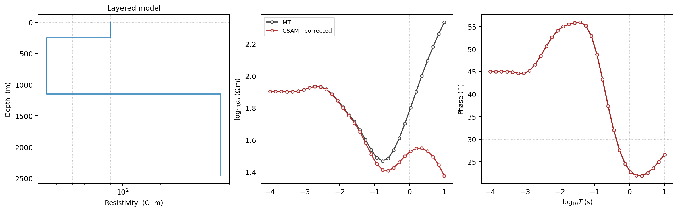
The CSAMT correction is strongest where \(r/\delta\) is small. At frequencies where the source is effectively far field, the corrected CSAMT curve returns to the MT-like response.

For MT and CSAMT 1-D responses:

• response.freqs has shape (n_freqs,);

• response.z has shape (n_freqs,) and is complex;

• response.rho_a has shape (n_freqs,);

• response.phase has shape (n_freqs,) in degrees;

• response.to_array() returns a one-dimensional feature vector.

When the model is one-dimensional, every surface station would see the same response. Use 2-D or 3-D grids when lateral geometry is part of the experiment.

16.4.4. 1-D TDEM Solver

TEM1DForward computes a central-loop step-off response for a layered earth. It uses time gates rather than frequencies as the primary output axis, but the underlying physics is still built frequency-first: for horizontal wavenumber \(\lambda\), the TE admittance recursion uses

(9)\[\nu_j^2 = \lambda^2 + i\omega\mu_0\sigma_j, \qquad Y^0_j = \frac{\nu_j}{i\omega\mu_0},\]

then integrates the reflected field with a Hankel-type kernel involving \(J_1(\lambda a)\), where \(a\) is the loop radius. The step-off decay is obtained with a cosine transform:

(10)\[\frac{dB_z}{dt}(t) \approx \frac{2}{\pi}\int_0^\infty \omega\,\Im\{H_z(\omega)\}\cos(\omega t)\,d\omega.\]

pyCSAMT delegates that Hankel-then-Fourier evaluation to empymod’s digital linear filters (Werthmüller, 2017) rather than a hand-rolled quadrature – an earlier from-scratch attempt at this exact integral did not converge reliably at realistic time ranges (its own frequency-domain kernel grew with frequency instead of decaying), which is a large part of why validated, peer-reviewed EM-transform libraries are worth depending on rather than re-deriving. The loop itself is represented internally as a small tangential electric-dipole segment at the loop radius, scaled by the loop’s circumference – exact by the axisymmetry of a horizontal circular loop, and the same construction empymod’s own gallery uses to reproduce Ward & Hohmann (1988)’s central-loop figures. TEM examples are still usually a little slower than MT1D ones simply because a full digital-filter transform does more work per time gate than a closed-form impedance recursion.

>>> import numpy as np

>>> from pycsamt.forward import LayeredModel, TEM1DForward

>>> model = LayeredModel(
...     resistivity=[60.0, 250.0, 900.0],
...     thickness=[120.0, 700.0],
... )

>>> times = np.logspace(-6, -3, 30)

>>> response = TEM1DForward(times=times, loop_radius=50.0).run(model)

>>> print(response.times.shape)
(30,)
>>> print(response.dBz_dt.shape)
(30,)
>>> print(response.to_array().shape)
(30,)
>>> print(np.all(response.dBz_dt > 0))
True

For TDEM responses:

• response.times has shape (n_times,);

• response.dBz_dt has shape (n_times,);

• response.to_array() returns a log-scaled decay feature vector by default.

A clean step-off response should stay single-signed and decay smoothly across the whole gate range – a real, physical sanity check worth plotting rather than only checking shapes:

>>> import matplotlib.pyplot as plt

>>> fig, ax = plt.subplots(figsize=(7, 5))
>>> _ = ax.loglog(times * 1e3, response.dBz_dt, "o-", ms=4, color="#1f77b4", label="dBz/dt")

>>> t_ref = times[-6:]
>>> ref = response.dBz_dt[-6] * (t_ref / times[-6]) ** (-2.5)
>>> _ = ax.loglog(t_ref * 1e3, ref, "--", color="0.4", lw=1.3, label=r"$t^{-5/2}$ reference")

>>> _ = ax.set_xlabel("time (ms)")
>>> _ = ax.set_ylabel(r"$dB_z/dt$ (arb. units)")
>>> _ = ax.set_title("TEM1DForward step-off decay -- 3-layer model")
>>> _ = ax.legend()
>>> _ = ax.grid(True, which="both", alpha=0.3)

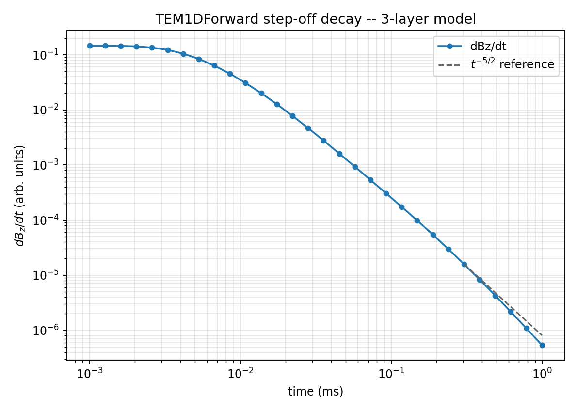
The dashed line is the classic conductive-halfspace late-time asymptote \(dB_z/dt \propto t^{-5/2}\) (Nabighian, 1979), anchored to the curve’s last point for comparison, not fitted to it.

The curve’s own late-time slope (a least-squares fit through the last third of the gates, in log-log space) comes out to about \(-2.70\) – close to but steeper than the ideal halfspace value of \(-2.5\), because the deep, resistive third layer (900 Ω·m below 820 m) is still shaping the decay rather than the response having settled into the true asymptotic regime. Early gates, by contrast, have a much shallower slope (about \(-0.30\) over the first eight points): the induced-current “smoke ring” has barely started diffusing outward and downward, so the field is still dominated by the near loop geometry rather than the earth’s conductivity structure. Use early gates to test shallow sensitivity and later gates to test deeper sensitivity; if the time range is too narrow, the inversion may fit the decay curve but remain insensitive to the target interval.

16.4.5. 2-D Profile Grid Concepts

pycsamt.forward.Grid2D stores a finite-difference grid for a profile. It contains:

• horizontal cell widths dx;

• vertical cell heights dz;

• cell resistivity matrix resistivity with shape (nz, nx);

• surface station x-positions x_stations;

• padding count n_pad;

• node and cell-centre coordinate helpers.

The grid uses depth-positive z coordinates. Resistivity is stored top-to-bottom and left-to-right. Stations must lie inside the grid extent. If n_pad is non-zero, the constructor arguments nx and nz describe the core model; the stored arrays are larger because padding cells are added on the left, right, and bottom. Thus a core grid with \(n_x^\mathrm{core}\) columns, \(n_z^\mathrm{core}\) rows, and \(p\) padding cells is stored approximately as

(11)\[n_x = n_x^\mathrm{core} + 2p,\qquad n_z = n_z^\mathrm{core} + p.\]

The exact physical width also grows because padded cell sizes are expanded by pad_factor.

The core region is the scientific model of interest. Padding cells are added on the left, right, and bottom to reduce boundary influence. The n_pad value records how many padding cells were added so plotting and interpretation tools can distinguish core cells from numerical buffer cells.

>>> import numpy as np

>>> from pycsamt.forward import Grid2D

>>> grid = Grid2D.halfspace(
...     rho=100.0,
...     nx=40,
...     nz=28,
...     x_max=8000.0,
...     z_max=5000.0,
...     n_pad=8,
...     pad_factor=1.3,
...     n_stations=12,
... )

>>> print(grid.resistivity.shape)
(36, 56)
>>> print(np.round(grid.x_stations, 1))
[ 6203.   6930.3  7657.5  8384.8  9112.1  9839.4 10566.6 11293.9 12021.2
 12748.5 13475.7 14203. ]
>>> print(grid.x_nodes[0], grid.x_nodes[-1])
0.0 20405.999163999997
>>> print(grid.core_resistivity.shape)
(28, 40)

16.4.6. 2-D Profile Grid Constructors

Use the constructor that matches the experiment you want to run.

Constructor	Purpose	Typical use
Grid2D.halfspace	Uniform background model.	Baseline checks, boundary tests, and solver sanity checks.
Grid2D.with_anomaly	Background with one rectangular resistive or conductive block.	Target detectability, station-spacing tests, and pseudosection training examples.
Grid2D.from_1d_layers	Laterally extends a layered model across a profile.	Compare 1-D and 2-D solvers, or build a simple starting model.
Grid2D.random	Randomized 2-D resistivity model.	Synthetic catalogues and stress tests.

A compact block-anomaly grid looks like this:

>>> from pycsamt.forward import Grid2D, MT2DForward

>>> grid = Grid2D.with_anomaly(
...     bg_rho=500.0,
...     anomaly_rho=5.0,
...     anomaly_bounds=(2000.0, 6000.0, 300.0, 1500.0),
...     nx=50,
...     nz=35,
...     x_max=10000.0,
...     z_max=6000.0,
...     n_pad=8,
...     n_stations=16,
... )

>>> response = MT2DForward(
...     freqs=[1.0, 10.0, 100.0],
...     grid=grid,
...     verbose=False,
... ).run()

anomaly_bounds are specified in core model coordinates as (x_lo, x_hi, z_lo, z_hi). The constructor internally accounts for padding when placing the anomaly into the full numerical grid.

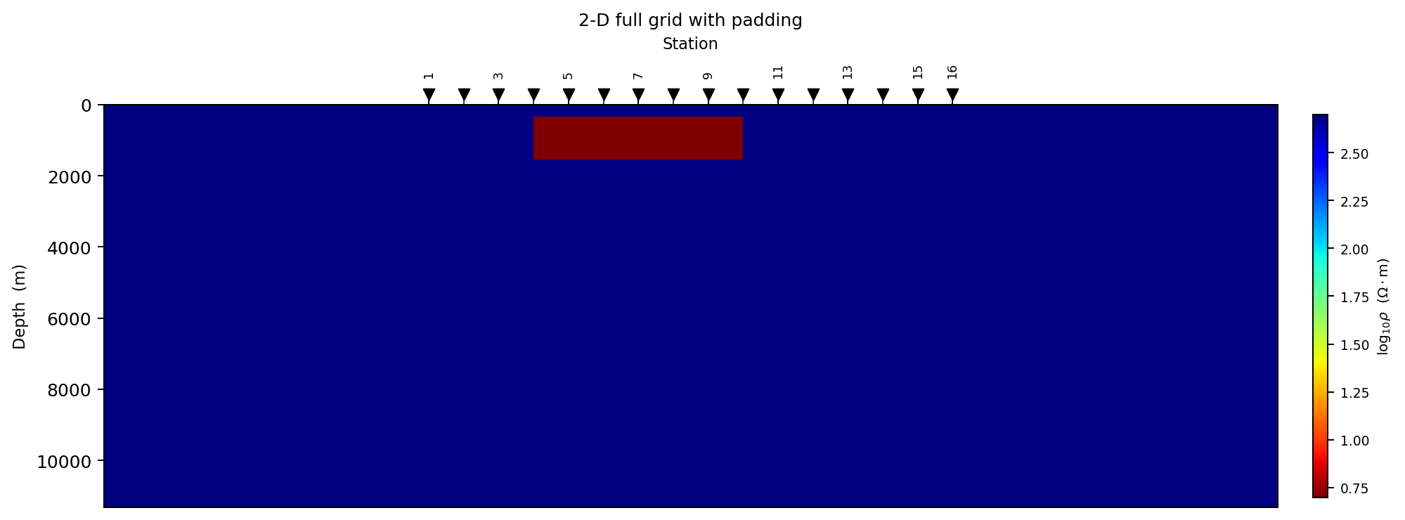
The full numerical grid includes padding cells. This view is useful for debugging boundary influence, not for geological interpretation.

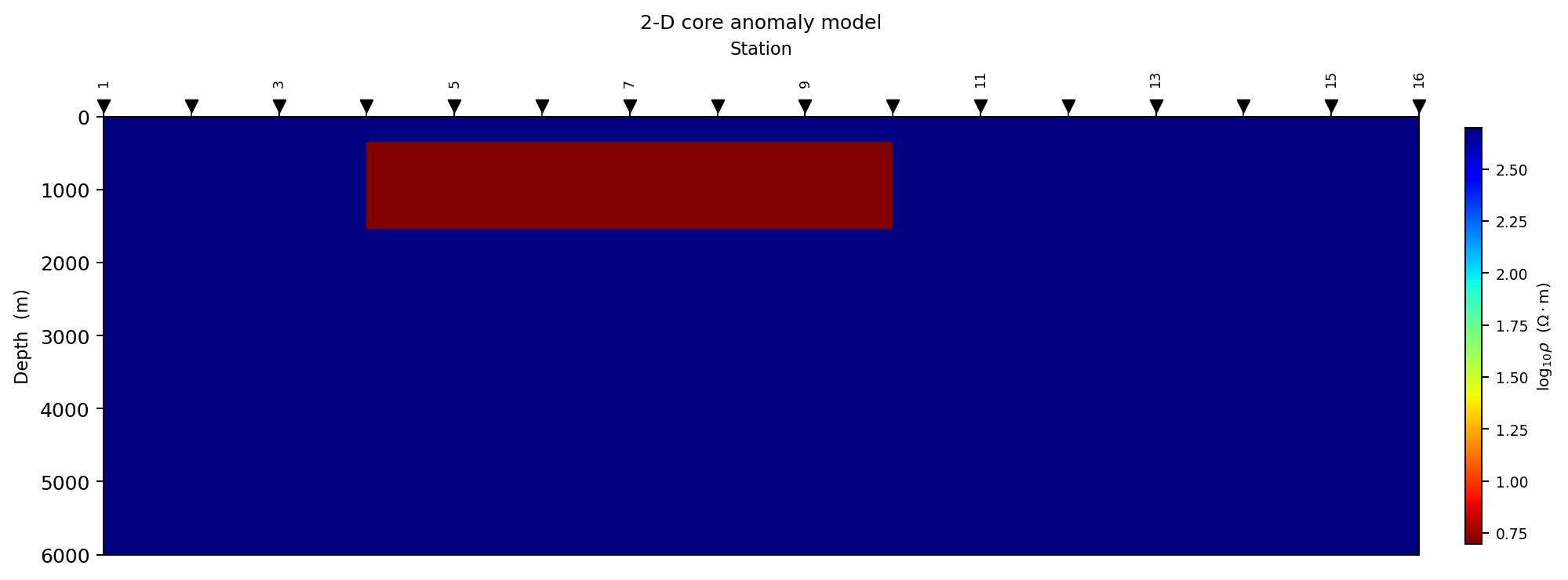
The clipped core view shows the scientific model: a conductive block inside a resistive background, sampled by surface stations.

16.4.7. 2-D MT Solver

MT2DForward solves the 2-D MT finite-difference problem for TE mode and TM mode. It returns a pycsamt.forward.ForwardResponse2D.

The code solves scalar frequency-domain problems on the grid nodes. For a conductivity field \(\sigma(x,z)=1/\rho(x,z)\), the TE unknown is \(E_y\); the TM unknown is \(H_y\). In compact continuous notation the operators can be read as

(12)\[\nabla^2 E_y - i\omega\mu_0\sigma E_y = 0,\]

and

(13)\[\nabla\cdot\left(\rho\,\nabla H_y\right) - i\omega\mu_0 H_y = 0.\]

The implementation discretises these equations with finite differences, enforces boundary values from 1-D edge-column responses, solves the sparse linear systems, then estimates surface impedance at the stations. The response conversion is the same impedance-to-observable relation used in 1-D: \(\rho_a=|Z|^2/(\omega\mu_0)\) and \(\phi=\arg Z\).

>>> station_0 = response.station_response(0)

>>> features_te = response.to_feature_array(
...     mode="te",
...     log_rho=True,
...     include_phase=True,
... )

>>> features_both = response.to_feature_array(
...     mode="both",
...     log_rho=True,
...     include_phase=True,
... )

>>> print(response.rho_a_te.shape)
(3, 16)
>>> print(response.phase_te.shape)
(3, 16)
>>> print(features_te.shape)
(16, 6)
>>> print(features_both.shape)
(16, 12)
>>> print(np.round(station_0["rho_a_te"], 2))
[156.17 424.41 607.92]
>>> print(np.round(station_0["phase_te"], 2))
[47.38 59.66 50.  ]

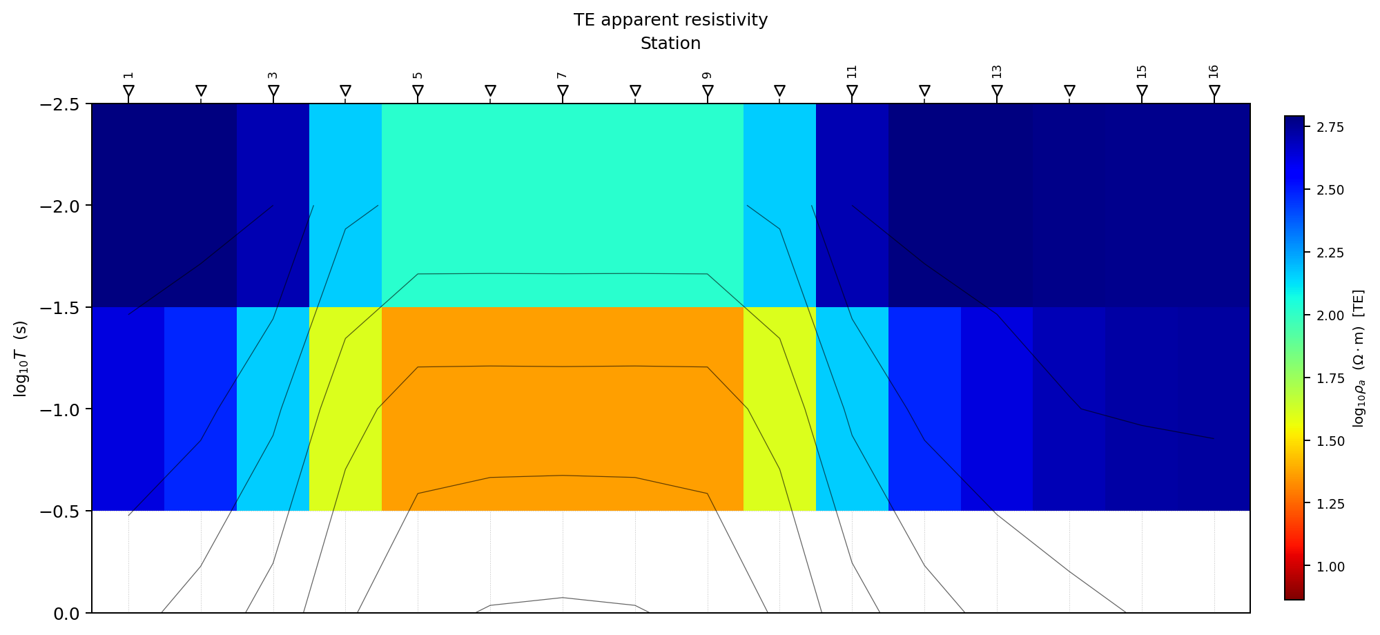
The pseudo-section is frequency-response geometry, not geology. It shows how the anomaly perturbs apparent resistivity across stations and periods.

Response array shapes are always frequency first:

Attribute	Shape	Meaning
response.freqs	(n_freqs,)	Frequency axis in Hz.
response.stations_x	(n_stations,)	Surface station positions.
response.zxy	(n_freqs, n_stations)	TE impedance component.
response.zyx	(n_freqs, n_stations)	TM impedance component.
response.rho_a_te	(n_freqs, n_stations)	TE apparent resistivity.
response.phase_te	(n_freqs, n_stations)	TE phase in degrees.
response.rho_a_tm	(n_freqs, n_stations)	TM apparent resistivity.
response.phase_tm	(n_freqs, n_stations)	TM phase in degrees.
response.to_feature_array()	(n_stations, n_features)	Station-first feature matrix for ML or downstream processing.

This difference is deliberate: physical response arrays are frequency-first, while feature matrices are station-first because each row is one training or analysis sample.

When passing a 2-D forward response to the inversion profile API, transpose the selected response arrays:

>>> inversion_data = {
...     "freqs": response.freqs,
...     "rho_a": response.rho_a_te.T,
...     "phase": response.phase_te.T,
...     "station_x": response.stations_x,
... }
>>> print(inversion_data["rho_a"].shape)
(16, 3)

16.4.8. 3-D Volume Grid Concepts

pycsamt.forward.Grid3D stores a 3-D resistivity volume and a 2-D station layout. It contains:

• cell widths dx, dy, and dz;

• resistivity with shape (nz, ny, nx);

• station coordinates stations_xy with shape (n_stations, 2);

• padding in x, y, and z;

• helpers that extract XZ and YZ slices for the quasi-3-D solver.

>>> from pycsamt.forward import Grid3D

>>> grid = Grid3D.halfspace(
...     rho=100.0,
...     nx=20,
...     ny=20,
...     nz=15,
...     x_max=8000.0,
...     y_max=8000.0,
...     z_max=4000.0,
...     n_pad=6,
...     nx_stations=5,
...     ny_stations=5,
... )

>>> print(grid.resistivity.shape)
(21, 32, 32)
>>> print(grid.stations_xy.shape)
(25, 2)

The regular station grid is created over the core model and shifted into the padded numerical coordinate system. As in 2-D, stations must lie inside the full grid extent. The stored resistivity array follows (nz, ny, nx) order, so depth is the first axis even though map coordinates are usually discussed as x and y first.

16.4.9. 3-D Volume Grid Constructors

The main constructors are:

Constructor	Purpose	Typical use
Grid3D.halfspace	Uniform 3-D background.	Baseline tensor and station-grid checks.
Grid3D.block_anomaly	Background with one 3-D rectangular block.	Survey design and quasi-3-D anomaly tests.
Grid3D.random_layered	Random laterally variable model.	Synthetic training data and robustness tests.

>>> from pycsamt.forward import Grid3D, MT3DForward

>>> grid = Grid3D.block_anomaly(
...     bg_rho=500.0,
...     anomaly_rho=20.0,
...     bounds=(2000.0, 6000.0, 2000.0, 6000.0, 300.0, 1500.0),
...     nx=20,
...     ny=20,
...     nz=15,
...     x_max=8000.0,
...     y_max=8000.0,
...     z_max=4000.0,
...     n_pad=6,
...     nx_stations=5,
...     ny_stations=5,
... )

>>> response = MT3DForward(
...     freqs=[1.0, 10.0, 100.0],
...     grid=grid,
...     verbose=False,
... ).run()

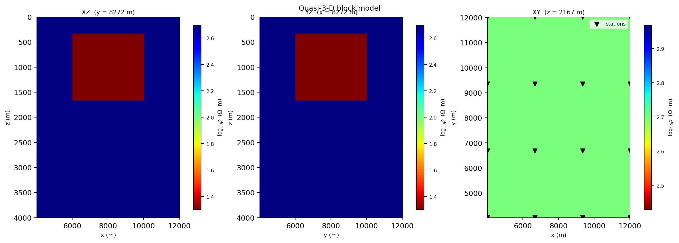
The 3-D grid is inspected through XZ, YZ, and XY slices. This is the fastest way to check whether anomaly bounds, depth range, and station coverage agree.

16.4.10. Quasi-3-D Solver

MT3DForward is a quasi-3-D MT solver. It does not claim to replace a full production 3-D modelling engine. Instead, it approximates tensor responses by extracting orthogonal 2-D slices from the 3-D grid and running MT2DForward on those slices.

Conceptually:

• XZ slices are grouped by station y-row;

• YZ slices are grouped by station x-column;

• TE and TM responses from both slice families are combined;

• off-diagonal tensor components Z_xy and Z_yx carry the main response;

• diagonal components Z_xx and Z_yy are represented as approximate tensor outputs and should be interpreted carefully.

The assembly can be read as a survey-design approximation. For station \(s=(x_s,y_s)\), the XZ slice through \(y_s\) gives one estimate of the profile response along \(x\); the YZ slice through \(x_s\) gives another estimate along \(y\). pyCSAMT stores the resulting tensor-like components as

(14)\[\begin{split}\mathbf{Z}_s(f) = \begin{bmatrix} Z_{xx,s}(f) & Z_{xy,s}(f) \\ Z_{yx,s}(f) & Z_{yy,s}(f) \end{bmatrix},\end{split}\]

then computes \(\rho_a\) and \(\phi\) component by component. The off-diagonal terms usually carry the most stable MT-style information; the diagonal terms are useful diagnostics but should not be over-interpreted as a validated full-3-D solution.

The output is pycsamt.forward.ForwardResponse3D.

>>> features = response.to_feature_array(
...     components="xy_yx",
...     log_rho=True,
...     include_phase=True,
... )

>>> all_components = response.to_feature_array(
...     components="all",
...     log_rho=True,
...     include_phase=False,
... )

>>> print(response.rho_a_xy.shape)
(3, 25)
>>> print(response.phase_xy.shape)
(3, 25)
>>> print(response.stations_xy.shape)
(25, 2)
>>> print(features.shape)
(25, 12)
>>> print(all_components.shape)
(25, 12)

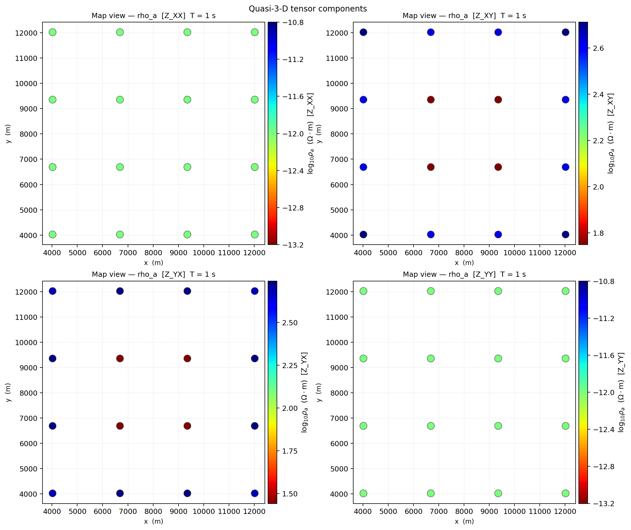
Tensor-component maps are best read comparatively: look for stable off-diagonal structure first, then treat diagonal panels as diagnostics of dimensionality and approximation limits.

As with the 2-D response, physical arrays are frequency-first: (n_freqs, n_stations). Feature arrays are station-first: (n_stations, n_features).

16.4.11. Grid Design Rules

Forward results are only as useful as the grid that produced them. Before trusting a response, check these points.

Positive resistivity

Every model cell must have strictly positive resistivity. The grid constructors validate this, but it is still worth checking after manual edits.

Station coverage

Stations must sit inside the grid. For profile experiments, station spacing should be small enough to sample the expected lateral anomaly signature.

Padding

Padding cells reduce boundary effects. Increase n_pad or pad_factor if the response changes noticeably when the model extent is increased.

Near-surface resolution

Shallow cells should resolve high-frequency or early-time sensitivity. A very coarse top layer can hide near-surface targets or create numerical artefacts.

Depth extent

The bottom of the grid should be deeper than the target and deeper than the main sensitivity range of the lowest frequencies or latest gates.

Frequency or time range

Do not rely on the solver to compensate for missing physics in the survey design. If the chosen axis cannot see the target, the inversion will not recover it reliably.

Dimensionality

Use 1-D models for layered checks, 2-D grids for profile structure, and quasi-3-D grids for survey design or synthetic AI catalogues. Move to Maxwell Adapter Layer’s validated adapters when the result needs a checkable accuracy claim, and further to native external backends through Overview when production 2-D or 3-D inversion files are required.

A useful numerical rule is to compare the target depth with the skin-depth range implied by the frequency axis – the same estimate from (4), evaluated once at each end of the swept band:

(15)\[\delta_\mathrm{min} \approx 503\sqrt{\rho_\mathrm{ref}/f_\mathrm{max}}, \qquad \delta_\mathrm{max} \approx 503\sqrt{\rho_\mathrm{ref}/f_\mathrm{min}}.\]

The grid bottom should usually extend beyond the deeper end of the sensitivity range, while the near-surface cells should be fine enough for the shallow end. This estimate is only a screening tool, but it catches many poor frequency-grid and depth-extent choices before a solver run.

A compact grid-check helper can be useful in notebooks. Re-building the earlier 2-D anomaly grid keeps this section runnable on its own, independent of the 3-D grids built in between:

>>> import numpy as np

>>> from pycsamt.forward import Grid2D

>>> grid2d = Grid2D.with_anomaly(
...     bg_rho=500.0,
...     anomaly_rho=5.0,
...     anomaly_bounds=(2000.0, 6000.0, 300.0, 1500.0),
...     nx=50,
...     nz=35,
...     x_max=10000.0,
...     z_max=6000.0,
...     n_pad=8,
...     n_stations=16,
... )

>>> def describe_grid2d(grid):
...     print(f"cells: nz={grid.nz}, nx={grid.nx}")
...     print(f"stations: {grid.n_stations}")
...     print(f"x extent: {grid.x_nodes[0]:.1f} to {grid.x_nodes[-1]:.1f} m")
...     print(f"z extent: {grid.z_nodes[0]:.1f} to {grid.z_nodes[-1]:.1f} m")
...     print(f"rho range: {np.nanmin(grid.resistivity):.3g} to "
...           f"{np.nanmax(grid.resistivity):.3g} ohm m")
...     print(f"padding cells: {grid.n_pad}")
...

>>> describe_grid2d(grid2d)
cells: nz=43, nx=66
stations: 16
x extent: 0.0 to 22406.0 m
z extent: 0.0 to 11316.9 m
rho range: 5 to 500 ohm m
padding cells: 8

16.4.12. Response Containers And Feature Arrays

Response containers preserve the physical arrays and also expose feature helpers for machine-learning and batch processing.

Response object	Physical shape	Feature shape
ForwardResponse	1-D arrays over frequency or time.	(n_features,).
ForwardResponse2D	(n_freqs, n_stations) arrays.	(n_stations, n_features).
ForwardResponse3D	(n_freqs, n_stations) arrays.	(n_stations, n_features).

Use physical arrays when preparing inversion data, plotting scientific responses, or checking units. Use feature arrays when training models, comparing many station responses, or building tabular downstream datasets.

16.4.13. Debugging Solver Experiments

When a forward response looks wrong, debug in this order:

1. Run a halfspace model first. A halfspace should produce smooth, stable responses.

2. Reduce the number of frequencies and stations until the experiment is easy to inspect.

3. Plot the grid with stations visible and confirm that the target is where you think it is.

4. Check whether the anomaly is inside the sensitivity range of the selected frequencies or time gates.

5. Increase padding and model extent. If the response changes strongly, the original grid was too small.

6. Compare a 2-D halfspace result with a 1-D MT response for the same resistivity.

7. Check array orientation before passing data to inversion or ML routines.

16.4.14. Next Pages

• Forward Configuration explains how configuration objects create grids and solvers.

• Synthetic Datasets And Noise explains how to generate many forward responses.

• Forward Plotting shows how to inspect models and responses.

• From Forward Modelling To Inversion explains how to pass synthetic responses to inversion workflows.