16.12. Synthetic Datasets And Noise#

Synthetic datasets are central to pyCSAMT v2. They are used for AI-assisted inversion, regression tests, solver benchmarks, survey design experiments, and documentation examples. A useful synthetic dataset is not just a collection of curves. It is a reproducible experiment that records:

the model family used to draw layered earth models;
the forward solver;
the frequency or time axis;
the feature vector transform;
the target vector layout;
the noise model;
the random seed;
the train, validation, and test dataset split.

The forward package currently provides two main dataset containers:

Container	Shape	Main use
`ForwardDataset`	`X` is `(n_samples, n_features)` and `y` is `(n_samples, n_params)`.	1-D MT, CSAMT, and TDEM model-response pairs.
`SurveyDataset3D`	`X` is `(n_surveys, n_stations, n_features)` and `y` is `(n_surveys, n_stations, n_params)`.	Pseudo-3-D multi-station datasets for spatial AI models.

The dataset generators are intentionally separate from the interactive forward solvers. Use individual solver objects when you need to inspect one model in detail. Use dataset generators when you need many reproducible samples. In mathematical terms, a 1-D generator repeatedly draws model parameters \(\mathbf{m}_k\) from a configured prior, evaluates a forward operator \(\mathbf{d}_k = F(\mathbf{m}_k)\), applies an optional noise operator \(\tilde{\mathbf{d}}_k = N(\mathbf{d}_k)\), and stores transformed pairs \((\mathbf{x}_k,\mathbf{y}_k)\) for learning or benchmarking.

16.12.1. 1-D Dataset Generation#

Use pycsamt.forward.generate_dataset() to create batches of independent 1-D forward responses. It supports solver="mt1d", solver="csamt1d", and solver="tem1d".

>>> import numpy as np

>>> from pycsamt.forward import generate_dataset

>>> dataset = generate_dataset(
...     solver="mt1d",
...     n_samples=1000,
...     freqs=np.logspace(-3, 4, 40),
...     n_layers=(3, 7),
...     rho_range=(1.0, 10000.0),
...     depth_max=3000.0,
...     noise_level=0.05,
...     noise_type="field",
...     include_phase=True,
...     seed=42,
...     n_jobs=1,
... )
>>> dataset.save("runs/forward/mt1d_dataset.npz")

Captured with the same recipe but a much smaller n_samples=12 (kept fast enough to actually run here, rather than illustrated only):

>>> dataset = generate_dataset(
...     solver="mt1d",
...     n_samples=12,
...     freqs=np.logspace(-3, 4, 40),
...     n_layers=(3, 7),
...     rho_range=(1.0, 10000.0),
...     depth_max=3000.0,
...     noise_level=0.05,
...     noise_type="field",
...     include_phase=True,
...     seed=42,
...     n_jobs=1,
...     verbose=False,
... )
>>> print(dataset)
ForwardDataset(n=12, n_features=80, n_params=13, solver='mt1d')
>>> print(dataset.X.shape)
(12, 80)
>>> print(dataset.y.shape)
(12, 13)
>>> print(dataset.freqs.shape)
(40,)
>>> print(np.unique(dataset.meta["n_layers"]))
[3 4 5 6 7]

Each sample is generated by:

drawing a pycsamt.forward.LayeredModel;
running the selected 1-D solver;
optionally applying noise;
converting the response into a feature vector;
converting the model into a target vector.

The generated dataset is a pycsamt.forward.ForwardDataset.

16.12.2. ForwardDataset Contract#

ForwardDataset stores the data needed for 1-D AI training or numerical experiments.

Attribute	Shape	Meaning
`X`	`(n_samples, n_features)`	Feature vectors generated from synthetic responses.
`y`	`(n_samples, n_params)`	Target model vectors. Shorter models are padded with `NaN`.
`freqs`	`(n_freqs,)` or `None`	Frequency axis for MT and CSAMT datasets.
`times`	`(n_times,)` or `None`	Time gates for TDEM datasets.
`meta`	structured array or `None`	Per-sample metadata, currently including layer count and noise level.
`solver`	string	Solver name used to generate the dataset.

For MT and CSAMT, the default feature vector contains log-scaled apparent resistivity and phase:

[log10(rho_a(f_0)), ..., log10(rho_a(f_n)),
 phase(f_0), ..., phase(f_n)]

When include_phase=False, only log10(rho_a) is used.

For TDEM, the feature vector contains log-scaled transient decay values:

1[log10(abs(dBz_dt(t_0))), ..., log10(abs(dBz_dt(t_n)))]

The target vector is produced from the layered earth model:

[log10(rho_0), log10(rho_1), ..., log10(rho_n),
 thickness_0, thickness_1, ..., thickness_n_minus_1]

When n_layers is a range, different samples can have different target lengths. If a model has \(L\) layers, its physical target length is \(2L-1\): \(L\) log-resistivities and \(L-1\) finite layer thicknesses. generate_dataset pads shorter targets with NaN so the final y array is rectangular. Training code should mask these padded values rather than treating them as physical targets.

16.12.3. Saving, Loading, And Splitting#

Datasets can be saved as compressed .npz files. Passing output=... to generate_dataset saves the dataset automatically, or you can call dataset.save yourself. Continuing with the 12-sample dataset from above, a fixed split seed gives a reproducible train/val/test partition:

>>> from pycsamt.forward import ForwardDataset

>>> dataset.save("runs/forward/mt1d_dataset.npz")

>>> loaded = ForwardDataset.load("runs/forward/mt1d_dataset.npz")

>>> train, val, test = loaded.split(
...     val_frac=0.1,
...     test_frac=0.1,
...     seed=0,
... )
>>> print(len(train), len(val), len(test))
10 1 1

Always split with a fixed seed when reporting model performance. This keeps the training, validation, and test partitions reproducible across machines.

16.12.4. Configuration-Driven Generation#

For repeatable studies, prefer a configuration file over a long script. The pycsamt.forward.ForwardConfig object records the same options accepted by generate_dataset and can write annotated templates.

>>> from pycsamt.forward import ForwardConfig, generate_dataset

>>> _ = ForwardConfig.write_template("runs/forward/mt1d_config.yml")

>>> cfg = ForwardConfig.from_file("runs/forward/mt1d_config.yml")
>>> cfg_kwargs = cfg.to_dataset_kwargs()
>>> cfg_kwargs["output"] = None
>>> cfg_dataset = generate_dataset(**cfg_kwargs)

This pattern makes it easier to archive the exact generation recipe alongside the resulting .npz file.

16.12.5. TDEM Datasets#

TDEM datasets use time gates and solver="tem1d". The target layout remains the same layered-earth vector, but dataset.times is populated instead of dataset.freqs.

>>> import numpy as np

>>> from pycsamt.forward import generate_dataset

>>> tdem_dataset = generate_dataset(
...     solver="tem1d",
...     n_samples=250,
...     times=np.logspace(-6, -3, 25),
...     n_layers=4,
...     rho_range=(5.0, 3000.0),
...     depth_max=1500.0,
...     loop_radius=40.0,
...     noise_level=0.03,
...     noise_type="gaussian",
...     seed=11,
...     n_jobs=1,
... )
>>> tdem_dataset.save("runs/forward/tem1d_dataset.npz")

Captured with the same recipe but n_samples=8:

>>> tdem_dataset = generate_dataset(
...     solver="tem1d",
...     n_samples=8,
...     times=np.logspace(-6, -3, 25),
...     n_layers=4,
...     rho_range=(5.0, 3000.0),
...     depth_max=1500.0,
...     loop_radius=40.0,
...     noise_level=0.03,
...     noise_type="gaussian",
...     seed=11,
...     n_jobs=1,
...     verbose=False,
... )
>>> print(tdem_dataset.times.shape)
(25,)
>>> print(tdem_dataset.X.shape)
(8, 25)
>>> print(tdem_dataset.y.shape)
(8, 7)

TDEM generation is usually slower than MT/CSAMT generation, since each sample runs the full empymod-backed digital-filter transform described in Solvers And Grids rather than a closed-form impedance recursion. Start with a small n_samples value when designing a new TDEM dataset recipe.

16.12.6. Geological Priors#

Instead of drawing all layer resistivities from a broad uniform range, you can ask generate_dataset to draw from a named geological prior. The underlying model generator uses pycsamt.forward.LayeredModel.from_geology().

>>> from pycsamt.forward import generate_dataset

>>> geothermal = generate_dataset(
...     solver="mt1d",
...     n_samples=500,
...     geology="geothermal",
...     noise_level=0.04,
...     noise_type="field",
...     seed=5,
... )

With a small n_samples=8 reproducibility check:

>>> geothermal = generate_dataset(
...     solver="mt1d",
...     n_samples=8,
...     geology="geothermal",
...     noise_level=0.04,
...     noise_type="field",
...     seed=5,
...     verbose=False,
... )
>>> print(geothermal)
ForwardDataset(n=8, n_features=60, n_params=9, solver='mt1d')
>>> print(geothermal.X.shape)
(8, 60)
>>> print(np.unique(geothermal.meta["n_layers"]))
[3 4 5]

Named priors are useful when the AI model should learn a specific geological setting rather than an overly broad synthetic universe. Keep a broad test set when possible, because overly narrow priors can make a model look better than it really is.

16.12.7. Noise Models#

Noise models make synthetic data more realistic and prevent AI models from learning only idealized solver curves. pyCSAMT keeps noise separate from the forward solver: first compute a clean physical response, then perturb it. If \(\mathbf{d}\) is the clean response and \(\epsilon\) is a random draw controlled by the seed, Gaussian-style noise can be read as \(\tilde{\mathbf{d}}=\mathbf{d}+\sigma\epsilon\) in transformed response space, while multiplicative noise perturbs values by a relative factor. The important reproducibility point is that the noise level, model type, and seed belong with the dataset, not only with the script that created it.

Noise model	How it behaves	Good use
`GaussianNoise`	Adds random perturbations in log-response space. For MT/CSAMT it perturbs `log10(rho_a)` and phase.	Baseline training, regression tests, quick robustness checks.
`MultiplicativeNoise`	Applies log-normal style perturbations, useful for values spanning many orders of magnitude.	Dynamic-range heavy data such as TDEM decays.
`FieldRealisticNoise`	Uses frequency-dependent noise with power-line harmonics and optional MT dead-band inflation.	MT/CSAMT training datasets intended to resemble field behaviour.

You can use named noise models through generate_dataset:

>>> field_dataset = generate_dataset(
...     solver="mt1d",
...     n_samples=1000,
...     noise_level=0.05,
...     noise_type="field",
...     seed=42,
... )

Or apply noise directly to a single response:

>>> import numpy as np

>>> from pycsamt.forward import FieldRealisticNoise, LayeredModel, MT1DForward

>>> model = LayeredModel([100.0, 20.0, 800.0], [300.0, 1000.0])
>>> response = MT1DForward(np.logspace(-3, 4, 40)).run(model)

>>> noise = FieldRealisticNoise(
...     base_level=0.03,
...     powerline_freq=50.0,
...     dead_band=True,
... )

>>> noisy_response = noise.apply(response, seed=42)
>>> profile = noise.noise_profile(response.freqs)
>>> print(profile.min(), profile.max())
0.03 0.15

A saved noise-profile plot makes the perturbation recipe auditable:

>>> import matplotlib.pyplot as plt

>>> fig, ax = plt.subplots(figsize=(7, 4.5))
>>> _ = ax.semilogx(response.freqs, profile, "-", color="#d62728", lw=1.6)
>>> _ = ax.axhline(
...     noise.base_level, ls="--", color="0.5", lw=1.0,
...     label=f"base level ({noise.base_level:.0%})",
... )
>>> _ = ax.set_xlabel("frequency (Hz)")
>>> _ = ax.set_ylabel("relative noise level")
>>> _ = ax.set_title("FieldRealisticNoise profile")
>>> _ = ax.legend()

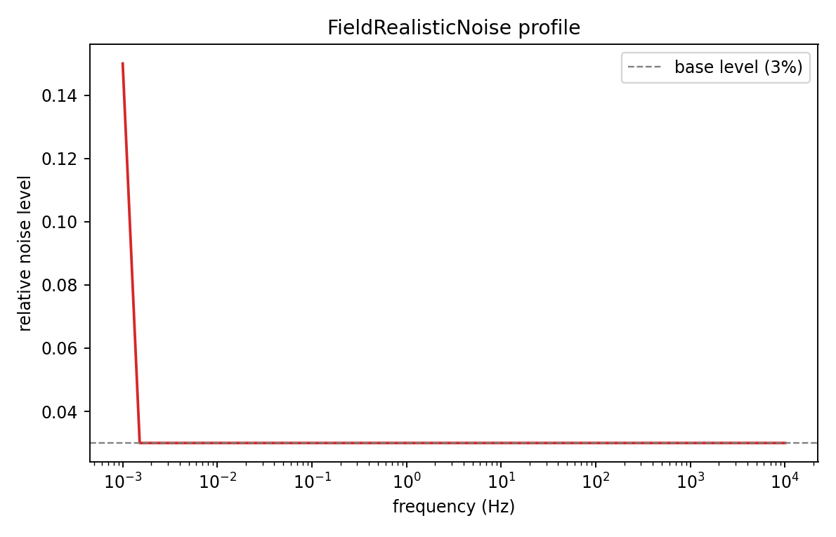
Every frequency sits at the 3% base level except the single lowest sample (0.001 Hz), which spikes to 15% – it falls inside dead_band_freq_range (0.0003-0.001 Hz by default), the low-frequency edge where natural-source MT signal strength genuinely drops off. None of the 40 sampled frequencies land near a 50 Hz power-line harmonic here, so that inflation mechanism happens not to fire for this particular frequency grid – a reminder that a noise profile is only as realistic as the axis it is evaluated on.#

FieldRealisticNoise requires a frequency-domain response. Use Gaussian or multiplicative noise for TDEM responses.

16.12.8. Clean And Noisy Dataset Pairs#

For benchmarking, it is often useful to generate one clean dataset and one noisy dataset with the same model draw settings. Use different output paths and keep the same seed.

>>> import numpy as np

>>> from pycsamt.forward import generate_dataset

>>> common = dict(
...     solver="mt1d",
...     n_samples=8,
...     freqs=np.logspace(-3, 4, 30),
...     n_layers=4,
...     rho_range=(1.0, 10000.0),
...     depth_max=2500.0,
...     include_phase=True,
...     seed=100,
...     n_jobs=1,
...     verbose=False,
... )

>>> clean = generate_dataset(**common, noise_level=0.0)
>>> noisy = generate_dataset(**common, noise_level=0.05, noise_type="gaussian")

The shared seed and draw settings are worth checking directly rather than assuming: the two calls should draw the exact same sequence of models, so only the features differ, not the targets:

>>> print("same targets:", np.array_equal(clean.y, noisy.y, equal_nan=True))
same targets: True
>>> print("same features:", np.array_equal(clean.X, noisy.X))
same features: False
>>> print("mean |X difference|:", round(float(np.abs(clean.X - noisy.X).mean()), 3))
mean |X difference|: 0.817

clean.y and noisy.y match element for element, confirming the model draw really is shared; clean.X and noisy.X differ, as expected, by roughly the injected noise level. This does not guarantee identical sample ordering if implementation details change in the future, but it is the intended reproducible pattern within the current generator – and it is the kind of assumption worth re-verifying rather than trusting on faith.

16.12.9. Pseudo-3-D Survey Datasets#

pycsamt.forward.generate_dataset_3d() creates multi-station survey datasets for graph-style or spatial AI models. It currently uses 1-D MT responses at each station, but draws station models from a spatially correlated Gaussian random field. This creates lateral structure in the target model while keeping the forward computation lightweight.

>>> from pycsamt.forward import generate_dataset_3d

>>> surveys = generate_dataset_3d(
...     solver="mt1d",
...     n_surveys=500,
...     n_stations=25,
...     n_layers=4,
...     extent=10000.0,
...     corr_length=2000.0,
...     noise_level=0.03,
...     noise_type="gaussian",
...     include_phase=True,
...     seed=7,
... )
>>> surveys.save("runs/forward/survey3d_dataset.npz")

Captured with four small surveys and nine stations:

>>> surveys = generate_dataset_3d(
...     solver="mt1d",
...     n_surveys=4,
...     n_stations=9,
...     n_layers=4,
...     extent=10000.0,
...     corr_length=2000.0,
...     noise_level=0.03,
...     noise_type="gaussian",
...     include_phase=True,
...     seed=7,
...     verbose=False,
... )
>>> print(surveys)
SurveyDataset3D(n_surveys=4, n_stations=9, n_features=60, n_params=7, solver='mt1d')
>>> print(surveys.X.shape)
(4, 9, 60)
>>> print(surveys.y.shape)
(4, 9, 7)
>>> print(surveys.coords.shape)
(9, 2)

SurveyDataset3D has this contract:

Attribute	Shape	Meaning
`X`	`(n_surveys, n_stations, n_features)`	Per-station feature vectors.
`y`	`(n_surveys, n_stations, n_params)`	Per-station layered model targets.
`coords`	`(n_stations, 2)`	Fixed station coordinates shared by all surveys.
`freqs`	`(n_freqs,)`	Frequency axis used by every station response.
`meta`	structured array	Per-survey correlation length and noise level.

All surveys share the same station layout. That is intentional: graph models can build one adjacency matrix from surveys.coords and reuse it for all survey realizations.

>>> from pycsamt.forward import SurveyDataset3D

>>> surveys.save("runs/forward/survey3d_dataset.npz")
>>> loaded = SurveyDataset3D.load("runs/forward/survey3d_dataset.npz")
>>> train, val, test = loaded.split(seed=0)
>>> print(train.X.shape)
(4, 9, 60)
>>> print(train.coords[:3])
[[    0.     0.]
 [ 5000.     0.]
 [10000.     0.]]

The corr_length parameter controls lateral smoothness. Values shorter than station spacing create rapidly varying station models. Values much longer than station spacing create smoother surveys.

16.12.10. 2-D And Quasi-3-D Solver Datasets#

The high-level batch generator is focused on 1-D and pseudo-3-D AI datasets. When you need full 2-D finite-difference or quasi-3-D response datasets, build a small custom loop around pycsamt.forward.Grid2D, pycsamt.forward.MT2DForward, pycsamt.forward.Grid3D, or pycsamt.forward.MT3DForward.

>>> import numpy as np

>>> from pycsamt.forward import Grid2D, MT2DForward

>>> freqs = np.logspace(-1, 3, 12)
>>> samples = []

>>> for seed in range(10):
...     grid = Grid2D.random(
...         nx=40,
...         nz=25,
...         x_max=6000.0,
...         z_max=3000.0,
...         n_stations=12,
...         seed=seed,
...     )
...     response = MT2DForward(freqs=freqs, grid=grid, verbose=False).run()
...     samples.append(response.to_feature_array(mode="both"))
...

>>> X = np.stack(samples, axis=0)

For three lightweight grid draws with eight stations, the same recipe gives:

>>> samples = []
>>> for seed in range(3):
...     grid = Grid2D.random(
...         nx=40,
...         nz=25,
...         x_max=6000.0,
...         z_max=3000.0,
...         n_stations=8,
...         seed=seed,
...     )
...     response = MT2DForward(freqs=freqs, grid=grid, verbose=False).run()
...     samples.append(response.to_feature_array(mode="both"))
...
>>> X = np.stack(samples, axis=0)
>>> print(X.shape)
(3, 8, 48)

This approach keeps large numerical experiments explicit. It also lets you store exactly the grid, response, and metadata needed by the study.

16.12.11. Dataset QA#

Before using a synthetic dataset for training, reporting, or benchmarking, perform basic quality assurance. Re-building the 12-sample MT1D dataset from the top of this page keeps this section runnable on its own:

>>> import numpy as np

>>> from pycsamt.forward import generate_dataset

>>> dataset = generate_dataset(
...     solver="mt1d",
...     n_samples=12,
...     freqs=np.logspace(-3, 4, 40),
...     n_layers=(3, 7),
...     rho_range=(1.0, 10000.0),
...     depth_max=3000.0,
...     noise_level=0.05,
...     noise_type="field",
...     include_phase=True,
...     seed=42,
...     n_jobs=1,
...     verbose=False,
... )

>>> def check_forward_dataset(dataset):
...     print(dataset)
...     print("X:", dataset.X.shape, dataset.X.dtype)
...     print("y:", dataset.y.shape, dataset.y.dtype)
...     print("finite X:", np.isfinite(dataset.X).all())
...     print("target NaN count:", np.isnan(dataset.y).sum())
...     if dataset.meta is not None:
...         print("layer counts:", np.unique(dataset.meta["n_layers"]))
...         print("noise levels:", np.unique(dataset.meta["noise_level"]))
...

>>> check_forward_dataset(dataset)
ForwardDataset(n=12, n_features=80, n_params=13, solver='mt1d')
X: (12, 80) float32
y: (12, 13) float32
finite X: True
target NaN count: 42
layer counts: [3 4 5 6 7]
noise levels: [0.05]

The check should be saved with the dataset archive.

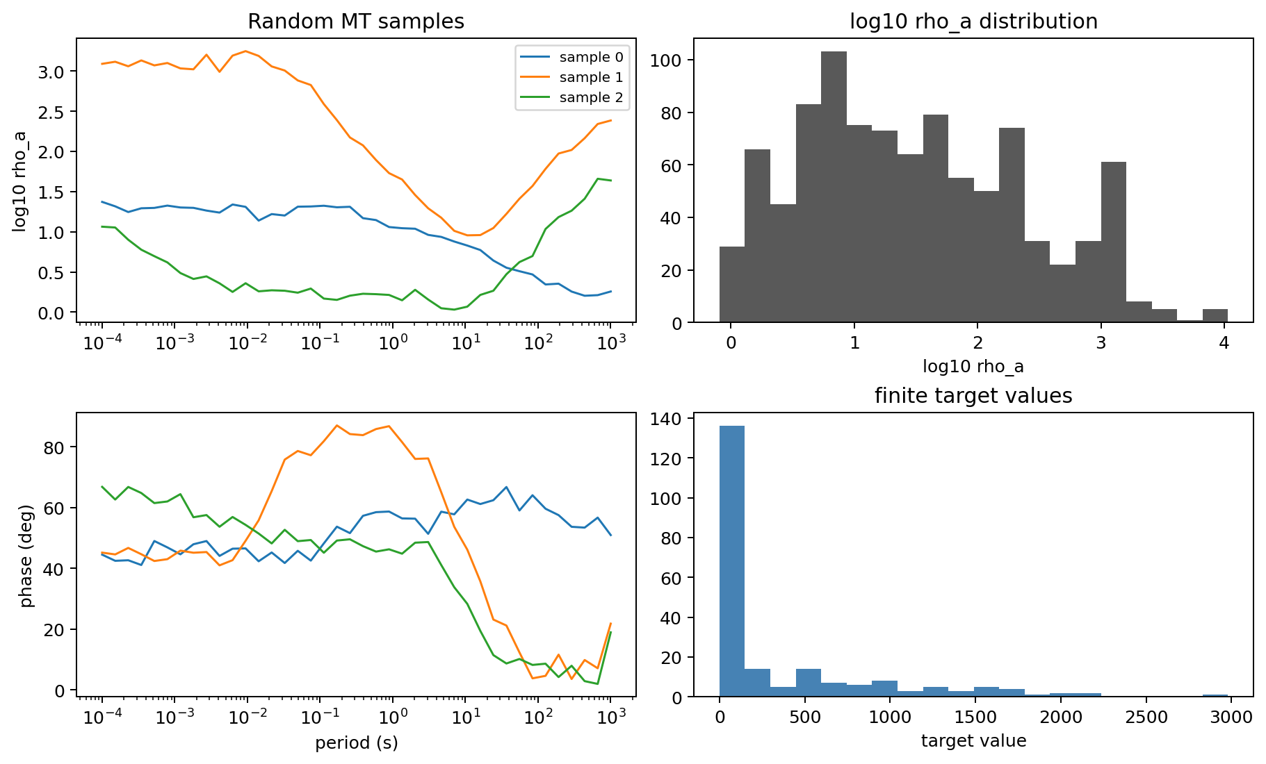
Synthetic dataset QA grid with sample curves and histograms. — A compact QA figure can show random response samples, feature distributions, and finite target values in one review artifact.#

Checklist:

plot random samples before training;
confirm there are no NaN or infinite values in X;
confirm NaN values in y are only padding;
verify the feature length expected by the model architecture;
inspect clean and noisy examples side by side;
keep frequency or time axes with the dataset;
keep train, validation, and test splits deterministic;
save the generation configuration and code version;
record the noise model and random seed.

16.12.12. Recommended Archive Layout#

A robust synthetic dataset directory should contain more than the .npz file.

synthetic_mt1d_v001/
  config.yml
  dataset.npz
  split_seed.txt
  qa_summary.txt
  plots/
    random_samples.png
    feature_histograms.png
    noise_profile.png
  notes.md

For production AI experiments, treat this directory as an immutable artifact. If you change the frequency grid, prior, noise model, target layout, or split seed, create a new dataset version.

16.12.13. Common Mistakes#

Training on clean data only: Clean data is useful for debugging, but a model trained only on clean curves usually fails on field-like data.
Ignoring padded target values: Variable-layer datasets contain NaN padding in y. Loss functions must mask those values.
Changing the frequency grid between train and test: The feature vector layout depends on the axis. A model trained on one frequency grid should not be evaluated on another without an explicit preprocessing strategy.
Using field noise for TDEM: FieldRealisticNoise is frequency-domain. Use Gaussian or multiplicative noise for TDEM.
Mixing station layouts in one graph dataset: SurveyDataset3D assumes a fixed station coordinate array so one adjacency matrix can be reused. Use separate datasets when layouts differ.

16.12.14. Next Pages#

Solvers And Grids explains the model containers and solver outputs.
Forward Plotting explains how to inspect generated samples.
From Forward Modelling To Inversion explains how to use synthetic responses in inversion recovery tests.