
9.3. AMT/CSAMT Edge Diagnostics#
Generic Edge QC covers what any edge diagnostics layer needs
regardless of method: finite coverage, spikes, decimation. The
pycsamt.iot.edge_amt module adds checks that are specific to
AMT, MT, and CSAMT field telemetry — the kind of
questions a generic coverage/spike screen cannot answer because they need
to look at the spectrum or at repeated impedance estimates rather than at
raw samples. These routines are intended for the edge side of a survey:
they run on short time windows, produce compact metrics, and help decide
whether a packet should be accepted, warned, or rejected before
downstream impedance tensor processing.
The examples below use synthetic data. No EDI or field logger file is required. The synthetic window is deliberately built with useful AMT-like energy, 50 Hz and 100 Hz powerline contamination, a clipped channel, a flat dropout interval, NaNs, and two sets of synthetic impedance windows, so that every check below has something real to catch.
9.3.1. What The Diagnostics Check#
Function |
Field question |
Typical action |
|---|---|---|
|
Are 50/60 Hz mains harmonics dominating this window? |
Warn or reject the packet, then inspect grounding and nearby power infrastructure. |
|
Is useful AMT-band energy above the noise floor? |
Prefer higher-SNR windows for transfer-function estimates. |
|
Is the ADC or logger rail clipping? |
Lower gain, check coil/electrode wiring, or discard saturated intervals. |
|
Do electric channels show high drift or high noise proxies? |
Re-seat electrodes, wet contacts, or review dipole wiring. |
|
Which target frequency bands are actually resolved? |
Mark missing bands before inversion or reporting. |
|
Are per-window impedance estimates repeatable? |
Keep stable windows and down-weight unstable windows. |
|
Did a channel go flat or contain gaps? |
Reject the affected interval and inspect sensor/logger health. |
9.3.2. Synthetic Edge Window#
Ex contains useful low-frequency energy plus 50 Hz and 100 Hz
powerline harmonics. Ey is also clipped to mimic an
overloaded ADC channel. Ex then receives a short flatline and
two NaNs to mimic a sensor dropout.
>>> import numpy as np
>>> sample_rate = 512.0
>>> n_samples = 8192
>>> t = np.arange(n_samples) / sample_rate
>>> rng = np.random.default_rng(42)
>>> ex = (
...     0.80 * np.sin(2 * np.pi * 7.5 * t)
...     + 0.35 * np.sin(2 * np.pi * 23.0 * t)
...     + 0.45 * np.sin(2 * np.pi * 50.0 * t)
...     + 0.18 * np.sin(2 * np.pi * 100.0 * t)
...     + 0.08 * rng.standard_normal(n_samples)
... )
>>> ey = (
...     0.65 * np.sin(2 * np.pi * 9.0 * t + 0.35)
...     + 0.22 * np.sin(2 * np.pi * 31.0 * t)
...     + 0.06 * rng.standard_normal(n_samples)
... )
>>> hx = (
...     0.32 * np.sin(2 * np.pi * 7.5 * t + 0.9)
...     + 0.05 * rng.standard_normal(n_samples)
... )
>>> ex_bad = ex.copy()
>>> ex_bad[2500:2560] = ex_bad[2499]
>>> ex_bad[6000] = np.nan
>>> ex_bad[6001] = np.nan
>>> ey_clipped = np.clip(2.6 * ey, -1.0, 1.0)
Before sending that window into the checks, it helps to know what each number means. The spectral routines work on a finite channel \(x_n\), sampled at rate \(f_s\); non-finite samples are linearly interpolated from the surrounding finite samples first (an edge run of NaNs takes the nearest finite value), so the two injected NaNs above do not silently zero out the spectrum around them. The one-sided power spectral density is computed with Welch averaging and is written below as \(P(f)\).
The mains check integrates the spectrum around each harmonic \(f_k = k f_m\), where \(f_m\) is 50 or 60 Hz:
The total contamination ratio is \(R = \sum_k r_k\), and a harmonic is
flagged when its own \(r_k\) is greater than or equal to the
configured threshold_ratio — a window can carry a modest total ratio
while still having one clearly flagged line, or vice versa. In this
example \(f_m = 50\) Hz and the 50 Hz line is expected to be the
dominant flagged harmonic. The same spectrum also gives the channel
SNR: useful in-band power is compared with the remaining spectral
power,
where \(f_1 = 4\) Hz and \(f_2 = 40\) Hz for the AMT band used below. The saturation check is more direct. With full-scale limit \(L\), a finite sample is clipped when \(|x_n| \ge L\), and the clip fraction is
The channel is marked saturated when \(c\) exceeds
max_clip_fraction. The contact check should be read in the same
field-practical spirit: check_contact_resistance is a contact
resistance proxy, not a direct injected-current measurement, and it uses
robust electric-channel noise/drift symptoms to flag channels that
deserve field inspection rather than a calibrated ohm value.
For frequency coverage, pyCSAMT takes the median positive PSD value as a noise floor \(P_{50}\). A frequency is resolved when
The lowest and highest resolved frequencies define \([f_\mathrm{low}, f_\mathrm{high}]\), and the number of covered decades is \(\log_{10}(f_\mathrm{high}/f_\mathrm{low})\). A target band counts as covered only when both of its bounds lie inside that resolved interval — a band that only partially overlaps the resolved range still counts as missing, which keeps the coverage fraction conservative. Impedance stability is checked on a stack of complex impedance tensor estimates \(Z_{ij}\) from repeated windows. For each frequency or component, pyCSAMT computes the magnitude coefficient of variation
and the standard deviation of the impedance phase \(\arg(Z)\) in
degrees. The returned summary is the average CV and average phase scatter
over the supplied impedance columns, and a window set is stable only when
both metrics stay below max_cv and max_phase_std_deg — a window
that is tight in magnitude but scattered in phase is still unstable.
Finally, detect_sensor_dropout scans the original sample sequence. It
reports the number of NaNs and the longest run of consecutive finite
samples satisfying \(|x_n - x_{n-1}| \le \epsilon\). A channel is a
dropout candidate if any NaN is present or if a flat run reaches
min_flat_run samples — the flatline in ex_bad above is exactly 60
samples long, deliberately built to clear a min_flat_run of 16.
9.3.3. Running The Edge Diagnostics#
The same window can be passed through the AMT-specific checks. The
target_bands argument says which bands the deployment cares about,
while signal_band_hz controls the SNR estimate.
>>> from pycsamt.iot import (
...     assess_impedance_stability, check_channel_saturation,
...     check_contact_resistance, detect_powerline_harmonics,
...     detect_sensor_dropout, estimate_channel_snr,
...     estimate_frequency_coverage,
... )
>>> harmonics = detect_powerline_harmonics(
...     ex_bad, sample_rate, mains_hz=50.0, n_harmonics=5,
...     threshold_ratio=0.02,
... )
>>> snr_ex = estimate_channel_snr(ex_bad, sample_rate, signal_band_hz=(4.0, 40.0))
>>> snr_hx = estimate_channel_snr(hx, sample_rate, signal_band_hz=(4.0, 40.0))
>>> saturation = check_channel_saturation(ey_clipped, limit=1.0, max_clip_fraction=0.01)
>>> contact = check_contact_resistance(
...     ex_bad, ey, sample_rate=sample_rate, noise_rms_threshold=0.45,
... )
>>> coverage = estimate_frequency_coverage(
...     ex_bad, sample_rate,
...     target_bands=[(4.0, 40.0), (40.0, 120.0), (120.0, 240.0)],
...     snr_floor_db=6.0,
... )
>>> dropout = detect_sensor_dropout(ex_bad, min_flat_run=16)
>>> z_stable = (1.0 + 0.45j) * (
...     1.0 + 0.03 * rng.standard_normal((16, 4))
... ) * np.exp(1j * np.deg2rad(1.5 * rng.standard_normal((16, 4))))
>>> z_unstable = (1.0 + 0.45j) * (
...     1.0 + 0.35 * rng.standard_normal((16, 4))
... ) * np.exp(1j * np.deg2rad(18.0 * rng.standard_normal((16, 4))))
>>> stable = assess_impedance_stability(z_stable)
>>> unstable = assess_impedance_stability(z_unstable)
>>> dominant = harmonics.dominant
>>> print(f"Powerline contaminated: {harmonics.contaminated}")
Powerline contaminated: True
>>> print(f"Dominant harmonic: {dominant.frequency_hz:.1f} Hz, ratio={dominant.power_ratio:.3f}")
Dominant harmonic: 50.0 Hz, ratio=0.200
>>> print(f"Total harmonic power ratio: {harmonics.total_ratio:.3f}")
Total harmonic power ratio: 0.232
>>> print(f"Ex SNR in 4-40 Hz band: {snr_ex:.2f} dB")
Ex SNR in 4-40 Hz band: 4.85 dB
>>> print(f"Hx SNR in 4-40 Hz band: {snr_hx:.2f} dB")
Hx SNR in 4-40 Hz band: 13.30 dB
>>> print(f"Ey clipped: {saturation['n_clipped']} of {saturation['n_samples']} ({100.0 * saturation['clip_fraction']:.1f}%), saturated={saturation['saturated']}")
Ey clipped: 4601 of 8192 (56.2%), saturated=True
>>> print(f"Contact proxy ok: {contact['ok']}, flags: {', '.join(contact['flags'])}")
Contact proxy ok: False, flags: ex_noise_above_threshold, ey_noise_above_threshold
>>> print(f"Frequency coverage: {coverage.f_low_hz:.2f}-{coverage.f_high_hz:.2f} Hz ({coverage.n_decades:.2f} decades)")
Frequency coverage: 2.00-102.00 Hz (1.71 decades)
>>> print(f"Target-band coverage fraction: {coverage.coverage_fraction:.2f}, missing: {coverage.missing_bands}")
Target-band coverage fraction: 0.33, missing: [(40.0, 120.0), (120.0, 240.0)]
>>> print(f"Dropout: {dropout['dropout']}, NaNs={dropout['n_nan']}, longest flat run={dropout['longest_flat_run']} samples")
Dropout: True, NaNs=2, longest flat run=61 samples
>>> print(f"Stable Z: {stable.stable} (CV={stable.cv_magnitude:.3f}, phase std={stable.phase_std_deg:.2f} deg)")
Stable Z: True (CV=0.026, phase std=1.60 deg)
>>> print(f"Unstable Z: {unstable.stable} (CV={unstable.cv_magnitude:.3f}, phase std={unstable.phase_std_deg:.2f} deg)")
Unstable Z: False (CV=0.308, phase std=18.63 deg)
Every printed line traces back to the numbers derived above. The dominant
harmonic sits at exactly 50 Hz with a 0.200 power ratio, comfortably over
the 0.02 threshold_ratio, and the second harmonic at 100 Hz — also
injected into ex — adds enough of the remaining ratio that the total
reaches 0.232; the three higher harmonics at 150, 200, and 250 Hz carry
essentially no power and stay unflagged, which is exactly what a spectrum
built from only two injected mains lines should show. Ex’s SNR sits at
4.85 dB because it is competing with those two harmonics inside its own
signal power, while Hx, which was built without any mains
contamination, reaches 13.30 dB in the same band. The longest flat
run of 61 rather than 60 samples is not an off-by-one error: the sample
immediately before the flatline (index 2499, whose value the flatline
repeats) already matches its neighbour, so the run detector correctly
counts one extra matching pair at the boundary.
9.3.4. The Diagnostic Figures#
The same variables can be plotted for review or embedded into an edge
report. The first figure shows the synthetic window and its live
power spectral density. The second condenses the key
quality control fractions and compares stable versus unstable
impedance windows. Neither plot has a dedicated plot_* helper in
pycsamt.iot.edge_amt — these diagnostics are metrics, not a
canned figure — so the plotting code below is written directly against
matplotlib using the values computed above.
>>> from pathlib import Path
>>> import matplotlib.pyplot as plt
>>> from pycsamt.iot import compute_live_spectra
>>> out_dir = Path("docs/source/images/user_guide/iot")
>>> out_dir.mkdir(parents=True, exist_ok=True)
>>> spectra = compute_live_spectra(ex_bad, sample_rate)
>>> freq = spectra["frequency_hz"]
>>> psd = spectra["psd"]
>>> fig, axes = plt.subplots(2, 1, figsize=(8.2, 5.8), constrained_layout=True)
>>> _ = axes[0].plot(t[:1600], ex_bad[:1600], lw=1.0, label="Ex synthetic")
>>> _ = axes[0].plot(t[:1600], ey[:1600], lw=0.9, alpha=0.75, label="Ey synthetic")
>>> _ = axes[0].set_xlabel("Time (s)")
>>> _ = axes[0].set_ylabel("Amplitude")
>>> _ = axes[0].set_title("Synthetic AMT edge window")
>>> _ = axes[0].legend(loc="upper right")
>>> axes[0].grid(alpha=0.25)
>>> _ = axes[1].semilogy(freq[1:], psd[1:], color="tab:blue")
>>> for peak in harmonics.peaks:
...     if peak.flagged:
...         _ = axes[1].axvline(peak.frequency_hz, color="tab:red", ls="--", lw=1.0, alpha=0.75)
>>> _ = axes[1].set_xlim(1, 180)
>>> _ = axes[1].set_xlabel("Frequency (Hz)")
>>> _ = axes[1].set_ylabel("PSD")
>>> _ = axes[1].set_title("Live spectrum with flagged mains harmonics")
>>> axes[1].grid(alpha=0.25, which="both")
>>> fig.savefig(out_dir / "user-guide-iot-amt-diagnostics-01.png", dpi=180)

>>> fig, axes = plt.subplots(1, 2, figsize=(8.2, 3.6), constrained_layout=True)
>>> _ = axes[0].bar(
...     ["Harmonic\nratio", "Ey clip\nfraction", "Missing\nband frac"],
...     [harmonics.total_ratio, saturation["clip_fraction"], 1.0 - coverage.coverage_fraction],
...     color=["tab:red", "tab:orange", "tab:purple"],
... )
>>> _ = axes[0].set_ylim(0, 1)
>>> _ = axes[0].set_ylabel("Fraction")
>>> _ = axes[0].set_title("Edge QC fractions")
>>> axes[0].grid(axis="y", alpha=0.25)
>>> _ = axes[1].bar(["Stable Z", "Unstable Z"], [stable.cv_magnitude, unstable.cv_magnitude], color=["tab:green", "tab:red"])
>>> _ = axes[1].axhline(0.15, color="0.25", ls="--", lw=1.0, label="max_cv")
>>> _ = axes[1].set_ylabel("Coefficient of variation")
>>> _ = axes[1].set_title("Impedance-window stability")
>>> _ = axes[1].legend(loc="upper left")
>>> axes[1].grid(axis="y", alpha=0.25)
>>> fig.savefig(out_dir / "user-guide-iot-amt-diagnostics-02.png", dpi=180)
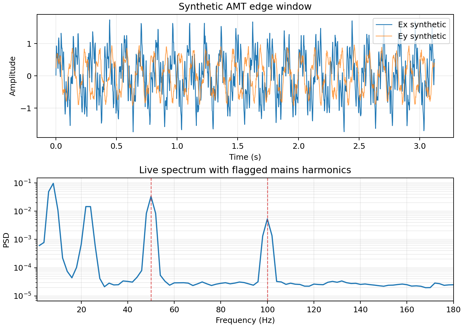
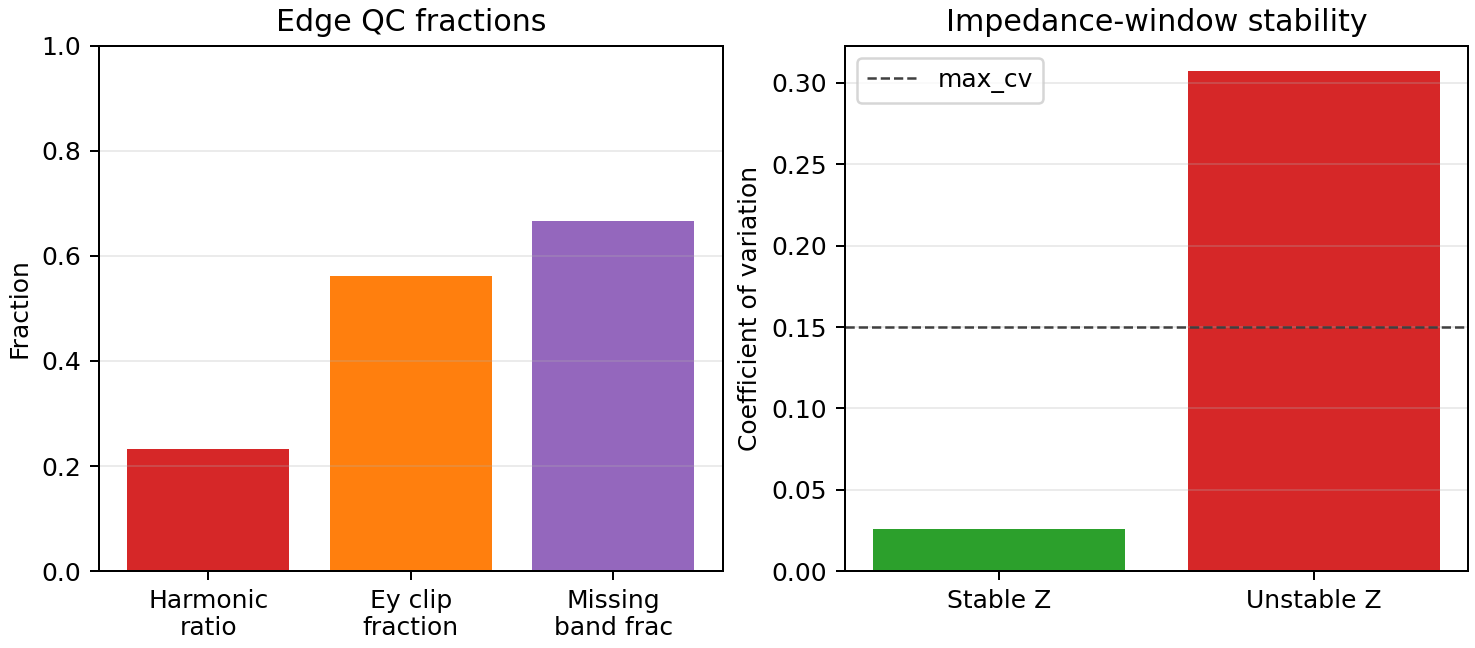
The top time series already looks noisy rather than obviously periodic,
because Ex is a sum of four sinusoids plus noise rather than one clean
tone; the mains contamination is invisible here and only becomes obvious
once the spectrum below it is in log scale. That spectrum shows two sharp
peaks marked by the red dashed lines at exactly 50 and 100 Hz, sitting
well above the broadband floor around \(10^{-5}\)-\(10^{-4}\) —
visual confirmation of the 0.200 and remaining harmonic ratios printed
above. In the fractions panel, the harmonic ratio (0.23) and the missing
target-band fraction (0.67, since two of the three requested bands were
not resolved) are both substantial, and the Ey clip fraction towers
over both at 0.56 — more than half the window is at the rail, which is by
itself already disqualifying for that channel regardless of what the
spectrum shows. The stability panel makes the max_cv threshold
concrete: the stable synthetic window sits far under the 0.15 dashed
line, while the unstable window, built with more than ten times the
per-sample scatter, clears it by a factor of two.
The synthetic packet built across this page should not be treated as a
clean acquisition window. The mains detector flags contamination because
the 50 Hz and 100 Hz bands carry a large fraction of the spectral power.
The clipped Ey channel is unusable for impedance estimation because
more than half of its samples are at the ADC limit. The
contact resistance proxy is a warning rather than a true
resistance measurement — passive AMT data cannot measure contact
resistance directly, but high drift and high channel noise are useful
field-side symptoms. The frequency coverage result says only one
of the three requested target bands is fully represented by this short
window; that does not mean the survey failed, only that this packet alone
should not be used to support the missing bands. The impedance-stability
comparison demonstrates the same principle one level downstream, at
transfer function level: low coefficient of variation and
low phase scatter mark windows worth keeping, while high magnitude and
phase scatter mark windows that should be down-weighted or rejected
before they reach an inversion.
9.3.5. Metrics In Telemetry#
In an IoT acquisition workflow, these diagnostics are usually attached to
qc packets or folded into the edge-processing result, the same way
Generic Edge QC attached generic coverage and spike metrics. A practical
edge policy might accept packets with finite data and stable impedance,
warn on mild mains contamination, and reject packets with saturation,
dropout, or severe missing-band coverage. The exact thresholds should be
survey-specific and recorded in the deployment manifest so that field
decisions remain reproducible. amt_edge_report()
bundles most of the checks on this page into one method-aware call, and
Method-Aware QC shows it gating powerline detection and target
bands from a declared acquisition method. When the source is an
operator-controlled transmitter rather than a passive plane wave, the
next page, Controlled-Source Edge QC (CSAMT / CSEM), adds the checks that only make sense
once there is a known source to compare the receiver against.