9.11. Clock Synchronisation#

Clock synchronisation is part of acquisition quality control. A station can have excellent electrodes and clean spectra, but poor timing still damages transfer function estimates, remote reference work, and any comparison between stations. The pycsamt.iot.sync helpers audit device clocks against a reference clock such as GPS.

The examples below use synthetic timestamp samples. That is intentional: synchronisation checks need paired local/reference clock samples, not EDI impedance files. The synthetic devices represent common field cases: one healthy GPS lock node, one drifting node, one node that lost GPS lock, and one badly drifting node.

9.11.1. What Is Measured#

offset_ms: Median local-reference clock offset in milliseconds.
drift_ppm: Linear clock drift in parts per million, estimated from offset change through time.
jitter_ms: Standard deviation of drift-corrected timing jitter residuals.
gps_lock: Whether the node reports active GPS/reference clock lock.
quality: A compact synchronisation quality grade: excellent, good, fair, poor, or unknown.

9.11.2. Synthetic Reference Samples#

The reference clock is sampled every 30 seconds for 10 minutes. Local device clocks are then offset, drifted, and jittered to create realistic audit cases.

>>> import numpy as np
>>> rng = np.random.default_rng(24)
>>> reference = np.arange(0.0, 600.0, 30.0)
>>> node_good = reference + 0.00035 + rng.normal(0.0, 0.00008, reference.size)
>>> node_drift = (
...     reference + 0.002 + 35e-6 * reference
...     + rng.normal(0.0, 0.00035, reference.size)
... )
>>> node_dropout = reference + 0.0035 + rng.normal(0.0, 0.0012, reference.size)
>>> node_bad = (
...     reference + 0.012 + 110e-6 * reference
...     + rng.normal(0.0, 0.002, reference.size)
... )
>>> print(reference.size)
20

The assessment that follows is based on paired finite samples \((l_i, r_i)\), where \(l_i\) is the local device timestamp and \(r_i\) is the reference timestamp, both in seconds. If the two input arrays have different lengths, pyCSAMT uses the shared prefix and drops non-finite pairs. For each surviving pair, the raw clock error is

\[e_i = l_i - r_i.\]

The reported offset is the median error in milliseconds:

\[\Delta t_\mathrm{ms} = 1000\,\operatorname{median}(e_i).\]

Using the median keeps one delayed or malformed timestamp from dominating the device status. Drift comes from fitting a straight line to error versus reference time,

\[e_i \approx a r_i + b,\]

and reporting \(10^6 a\) as clock drift in parts per million. Positive drift means the local clock is moving ahead of the reference; negative drift means it is falling behind. At least two distinct reference samples are required. Jitter is the scatter left after the fitted linear trend has been removed from millisecond errors:

\[j_\mathrm{ms} = \operatorname{std} \left(1000 e_i - (\alpha r_i + \beta)\right).\]

For only two samples, pyCSAMT falls back to the standard deviation of the raw millisecond offsets because a two-point line has no residual scatter. This makes timing jitter a short-window stability measure rather than another copy of absolute offset.

With those three values in hand, ClockSynchronizer.assess sets within_tolerance only when all configured finite checks pass:

\[|\Delta t_\mathrm{ms}| \le T,\quad |d_\mathrm{ppm}| \le D_\mathrm{max},\quad j_\mathrm{ms} \le J_\mathrm{max}.\]

The drift and jitter inequalities are skipped when the corresponding configuration value is None or the estimate is non-finite. The quality grade is intentionally stricter and easier to interpret in the field: with GPS lock, excellent requires \(|\Delta t| \le T\), \(|d| \le 2\) ppm, and \(j \le 0.5T\); good allows \(|d| \le 10\) ppm and \(j \le T\); fair allows \(|\Delta t| \le 5T\) and \(|d| \le 50\) ppm. Without GPS lock, quality is capped at fair when the offset is still within \(5T\), otherwise it is poor — a free-running clock can never grade above fair here, regardless of how small its offset happens to measure at one instant, because the lack of a reference lock means nothing guarantees it will stay that small.

GPS dropout is handled separately because a device can have an acceptable offset estimate and still lose reference support during acquisition. For lock flags \(g_i \in \{0,1\}\), the dropout helper reports

\[F_\mathrm{lock} = \frac{\sum_i g_i}{N}.\]

The status is ok only when \(F_\mathrm{lock}\) is at least min_lock_fraction. Consecutive unlocked samples are also counted as dropout events; when timestamps are supplied, the longest event is converted from samples to seconds.

9.11.3. Assess Individual Devices#

Use ClockSynchronizer when you already have local and reference timestamps for one device. The thresholds in SyncConfig define what counts as acceptable for this deployment.

>>> from pycsamt.iot import ClockSynchronizer, SyncConfig, sync_status_table
>>> config = SyncConfig(
...     tolerance_ms=1.0, reference="gps", max_drift_ppm=10.0, max_jitter_ms=1.0,
... )
>>> synchronizer = ClockSynchronizer(config)
>>> status = synchronizer.assess("l18-node-01", node_good, reference, gps_lock=True)
>>> table = sync_status_table(status)
>>> print(
...     table[
...         ["device_id", "offset_ms", "drift_ppm", "jitter_ms",
...          "within_tolerance", "gps_lock", "quality"]
...     ].to_string(index=False)
... )
  device_id  offset_ms  drift_ppm  jitter_ms  within_tolerance  gps_lock   quality
l18-node-01   0.344218  -0.004302   0.068069              True      True excellent

node_good was built with a constant 0.35 ms offset and no drift term at all, so an offset of 0.344 ms and a drift of essentially zero (-0.004 ppm) is the estimator recovering the construction almost exactly. That comfortably clears the excellent bar: offset under 1 ms, drift under 2 ppm, jitter under 0.5 ms.

9.11.4. Assess A Deployment#

For a deployment, keep one SyncStatus per node and turn the list into a table. This makes the failure mode visible: the second and fourth nodes exceed drift or offset limits, while the third node is capped at fair because GPS lock was lost.

>>> statuses = [
...     synchronizer.assess("l18-node-01", node_good, reference, gps_lock=True),
...     synchronizer.assess("l18-node-02", node_drift, reference, gps_lock=True),
...     synchronizer.assess("l18-node-03", node_dropout, reference, gps_lock=False),
...     synchronizer.assess("l18-node-04", node_bad, reference, gps_lock=True),
... ]
>>> table = sync_status_table(statuses)
>>> print(
...     table[
...         ["device_id", "offset_ms", "drift_ppm", "jitter_ms",
...          "within_tolerance", "gps_lock", "quality"]
...     ].to_string(index=False)
... )
  device_id  offset_ms  drift_ppm  jitter_ms  within_tolerance  gps_lock   quality
l18-node-01   0.344218  -0.004302   0.068069              True      True excellent
l18-node-02  12.276217  35.547894   0.392135             False      True      poor
l18-node-03   3.162285  -1.116131   1.383608             False     False      fair
l18-node-04  42.897972 108.638919   1.678547             False      True      poor

l18-node-02 and l18-node-04 both have GPS lock, yet both grade poor — lock alone does not certify quality once offset and drift blow through the thresholds by an order of magnitude or more (12.3 ms and 42.9 ms against a 1 ms tolerance). l18-node-03 is the more subtle case: its offset (3.16 ms) and drift (-1.12 ppm) are actually closer to acceptable than l18-node-02’s, and its jitter of 1.38 ms is only marginally over the 1 ms max_jitter_ms, but losing GPS lock caps it at fair regardless — the quality grade and within_tolerance are answering different questions, and here they disagree in an instructive way.

9.11.5. The Batch Helper#

When references are already arranged by device, use batch_assess_sync(). Each value can be a mapping with local, reference, and optional gps_lock fields.

>>> from pycsamt.iot import batch_assess_sync
>>> batch = batch_assess_sync(
...     {
...         "l18-node-01": {"local": node_good, "reference": reference, "gps_lock": True},
...         "l18-node-02": {"local": node_drift, "reference": reference, "gps_lock": True},
...     },
...     config=config,
... )
>>> print(batch[["device_id", "within_tolerance", "quality"]].to_string(index=False))
  device_id  within_tolerance   quality
l18-node-01              True excellent
l18-node-02             False      poor

batch_assess_sync is a thin convenience over the same ClockSynchronizer.assess call already used above — its two rows here match l18-node-01 and l18-node-02 from the deployment table exactly, just reached through a mapping instead of a list.

9.11.6. Detect GPS Dropout#

Use detect_gps_dropout() to summarise lock/unlock sequences. This is different from timestamp-pair assessment: it asks whether the device had enough reference clock support during the acquisition period, independent of what its offset/drift estimate says.

>>> from pycsamt.iot import detect_gps_dropout
>>> gps_lock = [True] * 8 + [False] * 3 + [True] * 6 + [False] * 2 + [True]
>>> dropout = detect_gps_dropout(
...     gps_lock, timestamps=np.arange(len(gps_lock)) * 30.0, min_lock_fraction=0.9,
... )
>>> for key in [
...     "n_samples", "n_locked", "lock_fraction", "n_dropout_events",
...     "longest_dropout_samples", "longest_dropout_s", "ok",
... ]:
...     value = dropout[key]
...     if isinstance(value, float):
...         print(f"{key}: {value:.3f}")
...     else:
...         print(f"{key}: {value}")
n_samples: 20
n_locked: 15
lock_fraction: 0.750
n_dropout_events: 2
longest_dropout_samples: 3
longest_dropout_s: 90.000
ok: False

The 20-sample sequence has two separate unlock runs — three samples, then two — for five unlocked samples total, giving lock_fraction=0.750. That is below the configured min_lock_fraction=0.9, so ok is False even though the device was locked for three quarters of the record; the longer of the two runs, three samples at 30-second spacing, converts to the reported 90-second longest_dropout_s.

9.11.7. The Synchronisation Figure#

The plotting helper summarises clock offset, clock drift, timing jitter, GPS lock, reference support, and quality grades in one figure.

>>> from pathlib import Path
>>> from pycsamt.iot import plot_sync_quality
>>> out_dir = Path("docs/source/images/user_guide/iot")
>>> out_dir.mkdir(parents=True, exist_ok=True)
>>> _ = plot_sync_quality(
...     statuses, tolerance_ms=config.tolerance_ms,
...     max_drift_ppm=config.max_drift_ppm, max_jitter_ms=config.max_jitter_ms,
...     figsize=(10.8, 7.2),
...     output_path=(out_dir / "user-guide-iot-clock-sync-01.png").as_posix(),
...     close=True,
... )

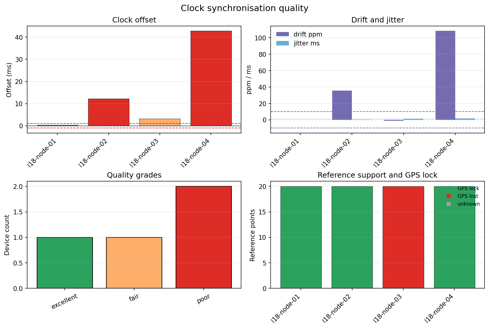
../../_images/user-guide-iot-clock-sync-01.png

The top-left panel is where the offset story becomes shape: three bars sit inside or barely past the ±1 ms dashed tolerance, but l18-node-04 towers over all of them at nearly 43 ms — more than 40 times the tolerance. The top-right panel tells a related but not identical story: l18-node-02’s drift bar (35.5 ppm) and l18-node-04’s (108.6 ppm) both clear the ±10 ppm dashed line by a wide margin, while l18-node-03’s drift is small enough to be barely visible — its problem, visible only in the bottom-right panel, is the red “GPS lost” bar, not drift or jitter at all. The quality-grades panel collapses all four devices into three bars: one excellent, one fair, two poor, matching the table above exactly. In a field workflow, store these status rows as sync telemetry packets or attach them to the acquisition manifest — the first node here is ready for timing-sensitive processing as is; the second and fourth should be corrected or excluded from time-critical windows; the third needs its GPS antenna or sky view checked even though its raw timing numbers look almost as good as the first node’s. That keeps the timing evidence next to the quality control, power, and station metadata used by later processing.