9.14. Simulation#

The IoT simulator creates deterministic field-like data for documentation, tests, demos, and pipeline development when hardware is not available. It can generate AMT channel windows, station/device inventories, telemetry packets, packet loss, GPS clock drift, and battery decay. Every simulator accepts a random seed argument so examples can be reproduced exactly. Every synthetic example elsewhere in this guide — the noisy half-space soundings, the multi-station sessions, the flaky uplinks — was built by hand from raw arrays and dictionaries; this page is the one place those same field-like inputs come from a single generator function instead.

These examples are synthetic data by design. They are not substitutes for real EDI or logger data; they are controlled inputs for testing the IoT layer around acquisition. Reproducibility comes from treating each simulator as a deterministic function of its arguments and seed: if the arguments and seed are unchanged, the generated samples, packets, and figures are unchanged.

9.14.1. Simulate AMT Channels#

Use simulate_amt_channel() to create one live channel window. The signal includes band-limited AMT-like energy, Gaussian noise, optional powerline harmonics, and optional dropout gaps. For a sample rate \(f_s\) and \(N\) samples, the time vector is \(t_i=i/f_s\). The simulator first builds a normalised signal from five random sinusoids,

\[s_i = \frac{\sum_{j=1}^{5} a_j \sin(2\pi f_j t_i + \phi_j)} {\operatorname{std}\left(\sum_{j=1}^{5} a_j \sin(2\pi f_j t_i + \phi_j)\right)} ,\]

where \(a_j\), \(f_j\), and \(\phi_j\) are drawn from the seeded random generator, with \(f_j\) uniform over \([0.05,\ f_s/4]\) — broadband by construction, not concentrated in any one target sub-band. A requested SNR of \(S_\mathrm{dB}\) is converted to \(S_\mathrm{lin}=10^{S_\mathrm{dB}/10}\), then white noise \(\epsilon_i \sim \mathcal{N}(0, 1/S_\mathrm{lin})\) is added. If a mains component is requested, the simulator adds \(\sum_{k=1}^{K} (A/k)\sin(2\pi k f_m t_i+\psi_k)\). Finally, the configured dropout rate replaces a reproducible number of contiguous samples with NaN values.

>>> import numpy as np
>>> from pycsamt.iot import (
...     EdgeProcessingConfig, EdgeProcessor, detect_powerline_harmonics,
...     estimate_channel_snr, simulate_amt_channel,
... )
>>> sample_rate = 256.0
>>> n_samples = 4096
>>> ex = simulate_amt_channel(
...     n_samples, sample_rate, snr_db=18.0, mains_hz=50.0,
...     powerline_amplitude=0.18, dropout_rate=0.015, seed=42,
... )
>>> ey = simulate_amt_channel(
...     n_samples, sample_rate, snr_db=12.0, mains_hz=50.0,
...     powerline_amplitude=0.06, dropout_rate=0.04, seed=43,
... )
>>> window = np.column_stack([ex, ey])
>>> harmonics = detect_powerline_harmonics(ex, sample_rate, mains_hz=50.0, threshold_ratio=0.02)
>>> snr_ex = estimate_channel_snr(ex, sample_rate, signal_band_hz=(2.0, 40.0))
>>> processor = EdgeProcessor(
...     EdgeProcessingConfig(
...         decimation=4, finite_threshold=0.90, warn_finite_threshold=0.98,
...         channel_names=["ex", "ey"], spike_threshold=5.0,
...     )
... )
>>> qc = processor.process(window)
>>> print(f"n_samples: {n_samples}")
n_samples: 4096
>>> print(f"sample_rate_hz: {sample_rate:.1f}")
sample_rate_hz: 256.0
>>> print(f"finite_coverage: {qc.metrics['finite_coverage']:.3f}")
finite_coverage: 0.975
>>> print(f"qc_decision: {qc.decision.value}")
qc_decision: warning
>>> print(f"ex_snr_2_40_hz_db: {snr_ex:.2f}")
ex_snr_2_40_hz_db: -6.76
>>> print(f"powerline_contaminated: {harmonics.contaminated}")
powerline_contaminated: True
>>> print(f"powerline_total_ratio: {harmonics.total_ratio:.3f}")
powerline_total_ratio: 0.371

ex_snr_2_40_hz_db reads as a poor -6.76 dB even though ex was built with a broadband snr_db=18.0 — the two numbers are not measuring the same thing. The requested 18 dB is the ratio of total signal power to total noise power across the whole spectrum, but the five random sinusoids that make up the signal are drawn uniformly up to \(f_s/4 = 64\) Hz, so most of that signal energy can easily land outside the narrow 2-40 Hz band the SNR estimator actually integrates over. A high requested SNR does not guarantee a high in-band estimate unless the signal energy happens to fall inside the band being checked.

9.14.2. Simulate One Station#

Use simulate_amt_station() when you need station metadata, a device config, channel arrays, and basic health/QC packets in one object. Each requested channel is generated with its own child seed from the station generator. The station-level finite coverage is the mean of per-channel finite fractions,

\[C = \frac{1}{M}\sum_{m=1}^{M} \frac{\#\{i : x_{m,i}\ \mathrm{is\ finite}\}}{N},\]

where \(M\) is the number of channels and \(N\) is the samples per channel. The synthetic QC packet is accepted when \(C \ge 0.95\) and the configured channel SNR is at least 6 dB; otherwise it is rejected. That makes station simulation useful for testing both clean and failed edge cases.

>>> from pycsamt.iot import simulate_amt_station
>>> station = simulate_amt_station(
...     "L18-S001", sample_rate=256.0, n_samples=1024, snr_db=16.0,
...     powerline_amplitude=0.1, dropout_rate=0.02, survey_id="SIM-L18",
...     profile="L18", position_m=0.0, seed=8,
... )
>>> print(f"station_id: {station['station'].station_id}")
station_id: L18-S001
>>> print(f"device_id: {station['device'].device_id}")
device_id: node-L18-S001
>>> print(f"channels: {', '.join(station['station'].channels)}")
channels: ex, ey, hx, hy
>>> print(f"packets: {len(station['packets'])}")
packets: 2
>>> print(f"qc_decision: {station['packets'][1].payload['decision']}")
qc_decision: accept

Unlike ex_snr_2_40_hz_db above, simulate_amt_station’s own accept/reject rule checks the configured snr_db directly rather than re-measuring an in-band estimate, so this station accepts on the strength of snr_db=16.0 \ge 6.0 and a coverage comfortably above 0.95 — the same broadband-versus-in-band gap noted above simply never enters this particular decision.

9.14.3. Simulate A Network#

Use simulate_iot_network() to create many stations across one or more profiles. With detail=True, the return value contains station dictionaries and a flat packet list. Use simulate_packet_loss() to drop a reproducible fraction of packets. Stations are assigned to profiles in round-robin order, and their profile positions advance by the configured spacing. Packet loss is a seeded Bernoulli keep/drop experiment: for packet \(p_i\), draw \(u_i \sim U(0,1)\) and keep the packet when \(u_i \ge q\), where \(q\) is dropout_rate. This means the exact kept packet inventory is reproducible, while still behaving like a lossy field link.

>>> from pycsamt.iot import (
...     packet_table, simulate_iot_network, simulate_packet_loss, telemetry_summary,
... )
>>> network = simulate_iot_network(
...     n_stations=6, profiles=["L18", "L22"], sample_rate=128.0, n_samples=512,
...     snr_db=14.0, dropout_rate=0.03, survey_id="SIM-WILLY",
...     station_spacing_m=50.0, seed=9, detail=True,
... )
>>> packets = network["packets"]
>>> kept = simulate_packet_loss(packets, dropout_rate=0.25, seed=10)
>>> print(f"original_packets: {len(packets)}")
original_packets: 12
>>> print(f"after_packet_loss: {len(kept)}")
after_packet_loss: 9
>>> print(
...     packet_table(kept)[
...         ["device_id", "kind", "timestamp", "payload_keys"]
...     ].head(6).to_string(index=False)
... )
    device_id   kind    timestamp                                                                payload_keys
node-L18-S001 health 1700000000.0                                    battery_v;firmware;station;temperature_c
node-L22-S001 health 1700000005.0                                    battery_v;firmware;station;temperature_c
node-L18-S002 health 1700000010.0                                    battery_v;firmware;station;temperature_c
node-L22-S002 health 1700000015.0                                    battery_v;firmware;station;temperature_c
node-L22-S002     qc 1700000019.0 accepted;channels;decision;finite_coverage;frequency_band_hz;method;station
node-L18-S003 health 1700000020.0                                    battery_v;firmware;station;temperature_c
>>> print(
...     telemetry_summary(kept)[
...         ["device_id", "topic", "n_packet"]
...     ].head(6).to_string(index=False)
... )
    device_id                                           topic  n_packet
node-L18-S001 pycsamt/SIM-WILLY/L18-S001/node-L18-S001/health         1
node-L18-S002 pycsamt/SIM-WILLY/L18-S002/node-L18-S002/health         1
node-L18-S003 pycsamt/SIM-WILLY/L18-S003/node-L18-S003/health         1
node-L18-S003     pycsamt/SIM-WILLY/L18-S003/node-L18-S003/qc         1
node-L22-S001 pycsamt/SIM-WILLY/L22-S001/node-L22-S001/health         1
node-L22-S002 pycsamt/SIM-WILLY/L22-S002/node-L22-S002/health         1

Six stations produce 12 packets (one health, one qc, each), and the seeded loss keeps 9 — but unevenly across kinds: all 6 health packets survive while only 3 of the 6 qc packets do. That split is an artefact of this particular seed and packet ordering, not a rule that favours one kind; a different seed would drop a different, still reproducible, subset.

9.14.4. Monitor Simulated Packets#

Simulated packets can be fed directly into the monitoring layer. This is useful when testing dashboard behavior or packet-loss handling before hardware exists. The same monitoring definitions used for real telemetry apply here: the monitoring status counts packets, estimates the edge acceptance rate, checks the maximum packet gap, and compares latency with the configured threshold. Because the packet stream is synthetic, a warning can be reproduced and debugged without waiting for a field outage.

>>> from pycsamt.iot import MonitoringConfig, TelemetryMonitor
>>> monitor = TelemetryMonitor(
...     MonitoringConfig(
...         method="amt", expected_interval_s=5.0, max_gap_s=20.0,
...         min_packet_success_rate=0.90, min_edge_acceptance_rate=0.80,
...         required_channels=["ex", "ey", "hx", "hy"],
...     )
... )
>>> status = monitor.assess(kept, now=1_700_000_080.0)
>>> print(f"level: {status.level.value}")
level: warning
>>> print(f"n_packet: {status.n_packet}")
n_packet: 9
>>> print(f"edge_acceptance_rate: {status.edge_acceptance_rate:.3f}")
edge_acceptance_rate: 1.000
>>> print(f"max_gap_s: {status.max_gap_s:.1f}")
max_gap_s: 5.0
>>> print(f"issues: {', '.join(status.issues) or '-'}")
issues: latency_above_threshold

Every one of the three surviving qc packets accepted, so edge_acceptance_rate is a perfect 1.000 and max_gap_s never approaches the 20-second limit — the only issue is latency_above_threshold, which traces back to now=1_700_000_080.0 being set well past the packets’ own timestamps. This is a status shaped entirely by how the monitor was asked to look at the stream, not by anything wrong with the simulated stations themselves.

9.14.5. Simulating GPS Drift#

Use simulate_gps_drift() to generate paired local and reference timestamps for synchronisation tests. The clock simulator starts from a reference clock time \(r_i=t_0+i\Delta t\) and creates a local timestamp

\[\ell_i = r_i + \frac{o_\mathrm{ms}}{1000} + d_\mathrm{ppm}\,10^{-6}(r_i-t_0) + \eta_i ,\]

where \(o_\mathrm{ms}\) is the initial offset, \(d_\mathrm{ppm}\) is the clock drift in PPM, and \(\eta_i \sim \mathcal{N}(0, \sigma_\mathrm{jitter}^2)\) is timing jitter in seconds. When simulated GPS lock is lost, the local clock receives an additional drift term to mimic free-running behavior.

>>> from pycsamt.iot import ClockSynchronizer, simulate_gps_drift
>>> gps = simulate_gps_drift(
...     120, sample_interval_s=1.0, drift_ppm=8.0, jitter_ms=0.25,
...     offset_ms=0.7, dropout_rate=0.1, seed=11,
... )
>>> sync = ClockSynchronizer().assess(
...     "l18-node-01", gps["local"], gps["reference"],
...     gps_lock=bool(np.mean(gps["gps_lock"]) > 0.9),
... )
>>> print(f"gps_lock_fraction: {np.mean(gps['gps_lock']):.3f}")
gps_lock_fraction: 0.892
>>> print(f"offset_ms: {sync.offset_ms:.3f}")
offset_ms: 1.214
>>> print(f"drift_ppm: {sync.drift_ppm:.3f}")
drift_ppm: 9.354
>>> print(f"jitter_ms: {sync.jitter_ms:.3f}")
jitter_ms: 0.254
>>> print(f"sync_quality: {sync.quality.value}")
sync_quality: fair

The recovered drift_ppm of 9.354 is close to but not exactly the requested drift_ppm=8.0 — the extra drift term samples where GPS lock is lost (10% of samples here) pulls the fitted slope up a little, which is the simulator’s own free-running-clock behaviour working as intended, not an estimation error. sync_quality lands on fair for a reason that has nothing to do with the lock fraction, though: the offset itself, 1.214 ms, already exceeds the default 1 ms tolerance, so neither excellent nor good was reachable regardless of GPS lock — both require offset within tolerance. With a lock fraction of 0.892, just under the 0.9 threshold this example checks, gps_lock is passed to assess as False too, which reaches the same fair grade through the free-running-clock branch instead. Either path lands on the same grade here, but for genuinely different reasons.

9.14.6. Simulating Battery Decay#

Use simulate_battery_decay() for power and monitoring demos. Battery decay uses an exponential sag from initial voltage \(V_0\) toward final voltage \(V_f\),

\[V_i = V_f + (V_0 - V_f)\exp(-2\alpha_i) + \nu_i, \qquad \alpha_i \in [0,1],\]

with small seeded voltage noise \(\nu_i\).

>>> from pycsamt.iot import simulate_battery_decay
>>> battery = simulate_battery_decay(120, initial_v=13.1, final_v=10.8, seed=12)
>>> print(f"battery_start_v: {battery[0]:.2f}")
battery_start_v: 13.10
>>> print(f"battery_end_v: {battery[-1]:.2f}")
battery_end_v: 11.06

battery_end_v lands at 11.06 V, not the requested final_v=10.8, because the exponential sag in the equation above only reaches \(V_f\) in the limit as \(\alpha_i \to \infty\); at \(\alpha_i = 1\) (the last sample) the curve has decayed to within \((V_0-V_f)e^{-2} \approx 0.31\) V of \(V_f\), and the small seeded noise term accounts for the rest of the gap.

9.14.7. The Simulation Figures#

The first figure shows channel time series and a spectrum with simulated mains contamination. The second shows the simulated network, packet counts after loss, clock drift, and battery decay. Both figures are generated from the same variables used in the examples above, so the visual output is tied to the captured text output rather than to a separate hidden dataset.

>>> from pathlib import Path
>>> import matplotlib.pyplot as plt
>>> out_dir = Path("docs/source/images/user_guide/iot")
>>> out_dir.mkdir(parents=True, exist_ok=True)
>>> t = np.arange(n_samples) / sample_rate
>>> freq = np.fft.rfftfreq(n_samples, d=1.0 / sample_rate)
>>> spec = np.abs(np.fft.rfft(np.nan_to_num(ex))) ** 2
>>> fig, axes = plt.subplots(2, 1, figsize=(9.0, 6.2), constrained_layout=True)
>>> _ = axes[0].plot(t[:1200], ex[:1200], lw=0.9, label="Ex")
>>> _ = axes[0].plot(t[:1200], ey[:1200], lw=0.9, alpha=0.75, label="Ey")
>>> _ = axes[0].set_title("Simulated AMT channels")
>>> _ = axes[0].set_xlabel("Time (s)")
>>> _ = axes[0].set_ylabel("Amplitude")
>>> _ = axes[0].legend(loc="upper right")
>>> axes[0].grid(alpha=0.25)
>>> _ = axes[1].semilogy(freq[1:], spec[1:], color="tab:blue")
>>> for peak in harmonics.peaks:
...     if peak.flagged:
...         _ = axes[1].axvline(peak.frequency_hz, color="tab:red", ls="--", lw=1.0)
>>> _ = axes[1].set_xlim(1.0, 128.0)
>>> _ = axes[1].set_title("Ex spectrum with simulated mains harmonics")
>>> _ = axes[1].set_xlabel("Frequency (Hz)")
>>> _ = axes[1].set_ylabel("Power")
>>> axes[1].grid(alpha=0.25, which="both")
>>> fig.savefig(out_dir / "user-guide-iot-simulation-01.png", dpi=180)
>>> plt.close(fig)
>>> fig, axes = plt.subplots(2, 2, figsize=(10.5, 7.0), constrained_layout=True)
>>> profiles = [item["station"].profile for item in network["stations"]]
>>> positions = [item["station"].position_m for item in network["stations"]]
>>> accepted = [item["packets"][1].payload["accepted"] for item in network["stations"]]
>>> colors = ["#2ca25f" if ok else "#de2d26" for ok in accepted]
>>> _ = axes[0, 0].scatter(positions, profiles, c=colors, s=90, edgecolor="black")
>>> _ = axes[0, 0].set_title("Simulated station network")
>>> _ = axes[0, 0].set_xlabel("Profile position (m)")
>>> _ = axes[0, 0].set_ylabel("Profile")
>>> axes[0, 0].grid(alpha=0.25)
>>> kinds = {}
>>> for packet in kept:
...     kinds[packet.kind.value] = kinds.get(packet.kind.value, 0) + 1
>>> _ = axes[0, 1].bar(kinds.keys(), kinds.values(), color="#756bb1")
>>> _ = axes[0, 1].set_title("Packets after simulated loss")
>>> _ = axes[0, 1].set_ylabel("Count")
>>> axes[0, 1].grid(axis="y", alpha=0.25)
>>> elapsed = gps["reference"] - gps["reference"][0]
>>> offset_ms = (gps["local"] - gps["reference"]) * 1000.0
>>> _ = axes[1, 0].plot(elapsed, offset_ms)
>>> _ = axes[1, 0].scatter(
...     elapsed[~gps["gps_lock"]], offset_ms[~gps["gps_lock"]],
...     color="tab:red", s=18, label="GPS lost",
... )
>>> _ = axes[1, 0].set_title("Simulated clock offset")
>>> _ = axes[1, 0].set_xlabel("Elapsed time (s)")
>>> _ = axes[1, 0].set_ylabel("Offset (ms)")
>>> _ = axes[1, 0].legend(loc="upper left")
>>> axes[1, 0].grid(alpha=0.25)
>>> _ = axes[1, 1].plot(np.arange(battery.size), battery, color="#2ca25f")
>>> _ = axes[1, 1].axhline(11.0, ls="--", color="#de2d26", label="low battery")
>>> _ = axes[1, 1].set_title("Simulated battery decay")
>>> _ = axes[1, 1].set_xlabel("Sample")
>>> _ = axes[1, 1].set_ylabel("Voltage")
>>> _ = axes[1, 1].legend(loc="upper right")
>>> axes[1, 1].grid(alpha=0.25)
>>> fig.savefig(out_dir / "user-guide-iot-simulation-02.png", dpi=180)
>>> plt.close(fig)

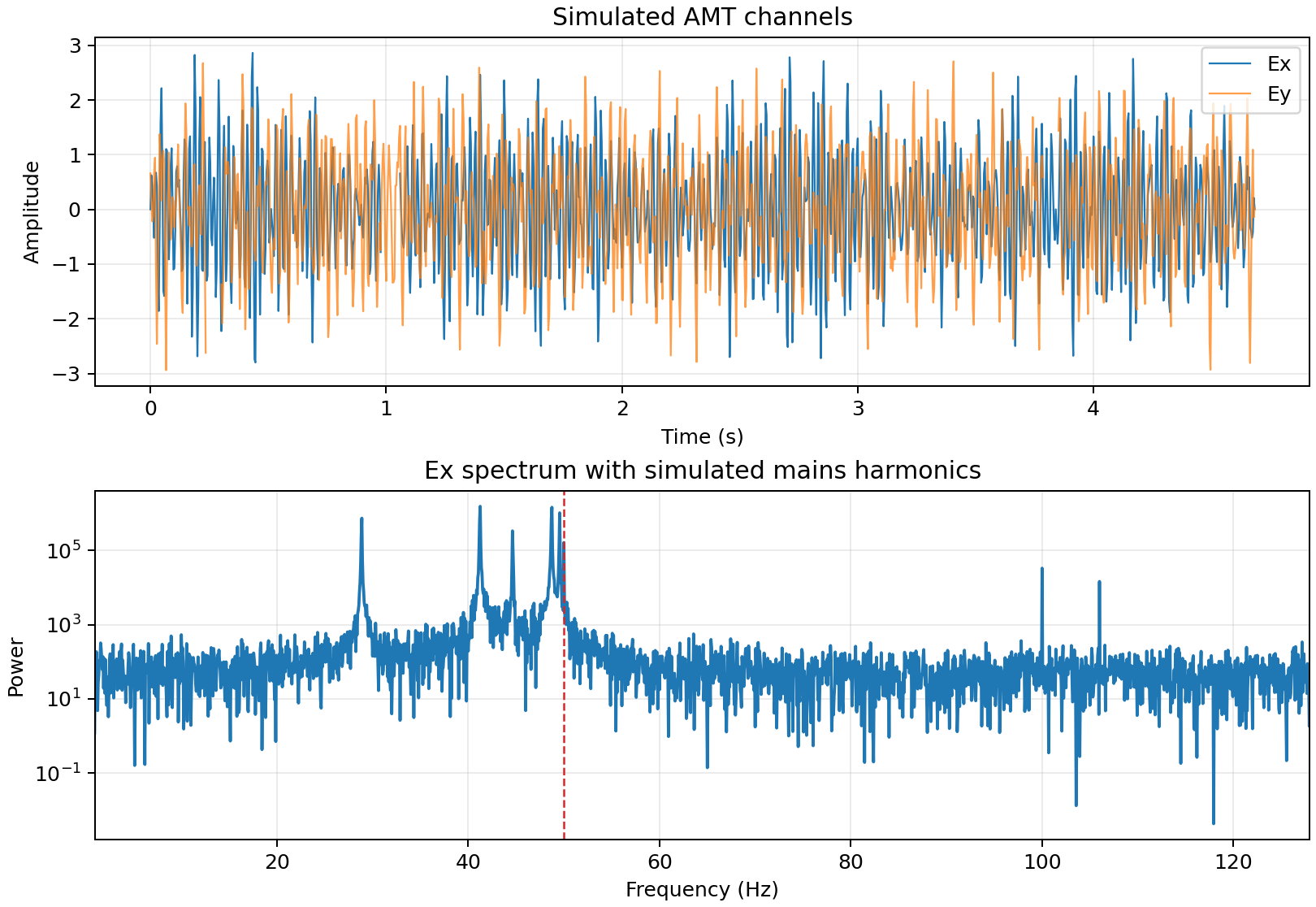
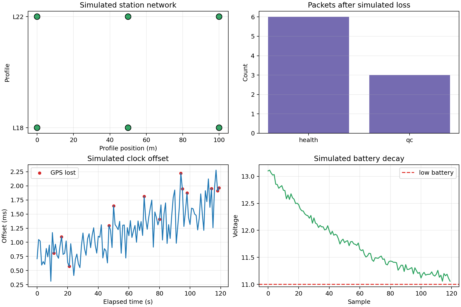
../../_images/user-guide-iot-simulation-01.png

../../_images/user-guide-iot-simulation-02.png

The top time series already looks noisy rather than obviously periodic, because Ex sums five broadband sinusoids plus noise plus a mains term, not one clean tone. The spectrum below it makes the mains contamination legible: a sharp peak sits exactly at the red dashed 50 Hz line — the one harmonic that actually cleared the 0.02 threshold — while a visible but unflagged second spike near 100 Hz shows the mains contamination extends further than the single flagged line reports; the remaining unlabelled peaks between roughly 25 and 50 Hz are simply where the five random signal sinusoids happened to land this seed, not mains-related at all. The station-network panel shows all six markers green, consistent with every station’s QC packet accepting above. The packet-count bar confirms the 6-versus-3 health/QC split from the network example — visibly uneven, not the roughly-even split a flat 25% loss rate might suggest. The clock-offset panel shows the offset trending upward over the two-minute window, with the red “GPS lost” points scattered throughout rather than clustered at one end — this simulator drops lock on a per-sample basis, not as one contiguous outage. The battery panel decays smoothly from just above 13 V toward the dashed 11 V line, with the small noise band visible throughout rather than a perfectly smooth exponential.

Simulation is useful because it makes edge cases reproducible with a single seed argument rather than a field outage. For production work, clearly label simulated data in reports and examples. Use simulation to test the IoT workflow shown throughout this guide, then replace simulated packets with real telemetry once field hardware is available.