
13.7. Computed Diagnostics#
The pycsamt.site.compute module provides lightweight station
diagnostics for EDI-like objects and site collections. These
functions do not modify the input data. They read impedance tensor,
frequency grid, and tipper arrays, then return compact
numerical summaries for quality control, survey preparation, and early
interpretation.
Use computed diagnostics before heavier processing when you need to answer questions such as:
does each station have a usable impedance tensor?
what geoelectric strike angle is suggested by the tensor structure?
what apparent resistivity is observed near a frequency of interest?
does phase vary smoothly across the band used for inversion?
is the tipper response small, large, missing, or spatially variable?
The common thread is reproducibility. Each diagnostic reduces the same recorded arrays to a small number of documented quantities, so another user can repeat the calculation from the same EDI files and check the same station table.
13.7.1. Input Contract#
The diagnostics accept either one EDI-like object or an iterable of EDI-like objects. In practice this means:
a
pycsamt.site.base.Sitescollection;a list, tuple, or other iterable of EDI-like objects.
The object must expose the data needed by the selected diagnostic:
Diagnostic |
Required arrays |
Missing-data behaviour |
|---|---|---|
|
Frequency vector and impedance tensor shaped |
Returns |
|
Frequency vector and impedance tensor shaped |
Returns |
|
Frequency vector and impedance tensor shaped |
Returns |
|
Frequency vector and tipper array shaped |
Returns |
For deterministic diagnostics on incomplete data, prepare the site first with
pycsamt.site.edit.fill_missing() or filter the survey with
pycsamt.site.selection.keep_finite_z().
13.7.2. Return Types#
The module follows one consistent rule:
Input |
Return value |
|---|---|
Single site |
A scalar or dictionary. |
Iterable of sites |
|
Iterable of sites with |
A pyCSAMT |
The following examples use a small synthetic EDI-like class so the printed
output is reproducible without relying on local survey files. Real workflows
usually replace the sites list with Sites.from_path("path/to/edi").
>>> import numpy as np

>>> from pycsamt.site.compute import (
...     phase_slope,
...     res_at_freq,
...     strike_estimate,
...     tipper_magnitude,
... )

>>> class ZBlock:
...     def __init__(self, freq, z):
...         self.freq = freq
...         self.z = z
...
>>> class TipBlock:
...     def __init__(self, tipper):
...         self.tipper = tipper
...
>>> class DemoSite:
...     def __init__(self, name, freq, z, tipper):
...         self.name = name
...         self.Z = ZBlock(freq, z)
...         self.Tip = TipBlock(tipper)
...
...     def get_section(self, name):
...         return getattr(self, name, None)
...
>>> freq = np.array([10.0, 30.0, 100.0, 300.0, 1000.0])
>>> base = (1 + 0.18j) * np.sqrt(freq / 100.0)
>>> logf = np.log10(freq / 100.0)

>>> def make_site(name, scale, diagonal, tip_scale, phase_xy, phase_yx):
...     z = np.zeros((freq.size, 2, 2), dtype=complex)
...     z[:, 0, 0] = diagonal * base
...     z[:, 1, 1] = -0.6 * diagonal * base
...     z[:, 0, 1] = (
...         scale * base * (1 + 0.05j) * np.exp(1j * phase_xy * logf)
...     )
...     z[:, 1, 0] = (
...         -0.85 * scale * base * (1 - 0.04j)
...         * np.exp(1j * phase_yx * logf)
...     )
...     tip = np.column_stack([
...         tip_scale * (0.12 + 0.02j) * np.ones(freq.size),
...         tip_scale * (0.06 - 0.01j) * np.linspace(1.0, 1.4, freq.size),
...     ])
...     return DemoSite(name, freq, z, tip)
...
>>> sites = [
...     make_site("S01", 1.00, 0.08, 1.0, 0.12, -0.08),
...     make_site("S02", 1.25, 0.15, 1.6, 0.20, -0.13),
...     make_site("S03", 0.75, 0.04, 0.7, -0.10, 0.16),
... ]

>>> print("single strike:", strike_estimate(sites[0], method="swift", api=False))
single strike: 72.0
>>> print(
...     "single rho:",
...     {k: round(v, 3) for k, v in res_at_freq(
...         sites[0], 150.0, how="nearest", api=False
...     ).items()},
... )
single rho: {'res_xy': 1310.819, 'res_yx': 946.216, 'f_used': 100.0}
>>> print(
...     "single slope:",
...     {k: round(v, 3) for k, v in phase_slope(
...         sites[0], band=(10.0, 1000.0), api=False
...     ).items()},
... )
single slope: {'slope_xy': 6.875, 'slope_yx': -4.584}
>>> print(
...     "single tipper:",
...     {k: round(v, 3) for k, v in tipper_magnitude(
...         sites[0], api=False
...     ).items()},
... )
single tipper: {'mean': 0.142, 'median': 0.142, 'max': 0.148}
13.7.3. Diagnostic Map#
Function |
Output |
Main use |
|---|---|---|
|
|
Quick geoelectric strike estimate for tensor rotation checks and 2-D assumption screening. |
|
|
Compare stations at one frequency, select target frequency slices, or build compact QC tables. |
|
|
Detect abrupt phase behaviour, band-edge problems, or unstable curves. |
|
Mean, median, max, or per-frequency tipper magnitude. |
Evaluate vertical magnetic transfer response and possible 3-D structure indicators. |
13.7.4. Strike Estimate#
strike_estimate() estimates a 2-D geoelectric strike angle from the
impedance tensor. The tensor at one frequency is
In an ideal 2-D coordinate frame the diagonal terms are small and the off-diagonal components carry the TE/TM response. The Swift-style diagnostic therefore rotates the tensor by a trial angle \(\theta\),
and chooses the angle that makes the rotated diagonal energy smallest:
The median over frequency makes the screening value less sensitive to one
noisy band than a simple sum would be. The result is still a diagnostic, not a
final structural interpretation; compare neighbouring stations before rotating
an entire line with pycsamt.site.edit.rotate() or
pycsamt.site.edit.rotate_all().
The minimization in equation (3) has the usual 90-degree MT ambiguity: exchanging the two horizontal axes describes the same pair of principal directions. Compare angles modulo 90 degrees and use geological continuity, profile direction, and neighbouring stations to decide which direction should be called strike.
>>> strike_table = strike_estimate(sites, method="swift", api=False)
>>> print(strike_table.to_string(index=False))
station method  theta_deg
    S01  swift       72.0
    S02  swift      156.0
    S03  swift       79.0
method="groom" currently uses the same lightweight criterion as
"swift". method="phase_diff" is a coarse fallback that returns either
0 or 90 degrees from the relative median magnitudes of \(Z_{xy}\) and
\(Z_{yx}\).
13.7.5. Apparent Resistivity At One Frequency#
res_at_freq() evaluates apparent resistivity for \(Z_{xy}\) and
\(Z_{yx}\) at a requested frequency. For angular frequency
\(\omega = 2\pi f\), pyCSAMT uses
where \(Z(f)\) is the selected complex impedance component, \(\mu_0\) is magnetic permeability, and \(f\) is frequency in Hz. Because \(|Z|^2\) is used, the sign difference between \(Z_{xy}\) and \(Z_{yx}\) does not by itself change \(\rho_a\); differences in their amplitudes do.
Two frequency-selection modes are available:
how="nearest"Select the nearest available native frequency and report that value in
f_used.how="interp"Compute resistivity at all native frequencies, then interpolate to the requested frequency using linear interpolation in frequency.
>>> near = res_at_freq(sites, 150.0, how="nearest", api=False)
>>> interp = res_at_freq(sites, 150.0, how="interp", api=False)

>>> print(near.round(3).to_string(index=False))
station   res_xy   res_yx  f_used
    S01 1310.819  946.216   100.0
    S02 2048.154 1478.463   100.0
    S03  737.336  532.247   100.0
>>> print(interp.round(3).to_string(index=False))
station   res_xy   res_yx  f_used
    S01 1310.819  946.216   150.0
    S02 2048.154 1478.463   150.0
    S03  737.336  532.247   150.0
Use nearest when preserving the exact sampled frequency axis matters. Use
interp when stations have slightly different grids and you need one common
comparison frequency across the survey.
The resistivity columns happen to be identical in these two tables because
the synthetic impedance amplitude is proportional to \(\sqrt f\); after
division by \(f\) in equation
(4), its apparent resistivity is
constant. The different f_used values still expose the distinct selection
rules. A field response that varies with frequency will generally produce
different interpolated values as well.
13.7.6. Phase Slope#
phase_slope() summarizes how phase changes across a frequency band. For
each off-diagonal component it computes
then fits a straight line against logarithmic frequency:
The reported slope \(a\) is measured in degrees per frequency decade. A value near zero means phase is nearly flat over the selected band; a large positive or negative value means the component changes rapidly with frequency and should be inspected before inversion.
>>> slopes = phase_slope(sites, band=(10.0, 1000.0), api=False)
>>> steep = slopes[
...     slopes["slope_xy"].abs().gt(30.0)
...     | slopes["slope_yx"].abs().gt(30.0)
... ]

>>> print(slopes.round(3).to_string(index=False))
station  slope_xy  slope_yx
    S01     6.875    -4.584
    S02    11.459    -7.448
    S03    -5.730  -133.479
>>> print("steep rows:", len(steep))
steep rows: 1
The function does not unwrap phase. If phase wraps are important for your
dataset, inspect the curves directly before treating the slope as a physical
trend. In particular, the large negative S03 value is produced by a phase
branch crossing rather than a smooth 133-degree-per-decade physical change.
Unwrap or mask that component before fitting if continuity across the branch
is scientifically justified.
13.7.7. Tipper Magnitude#
tipper_magnitude() computes the magnitude of the complex tipper vector:
The square root combines the two horizontal transfer components into one
station-level amplitude per frequency. By default pyCSAMT summarizes those
amplitudes with mean, median, and maximum values; set per_freq=True when
the frequency-by-frequency curve is needed.
>>> summary = tipper_magnitude(sites, api=False)
>>> long_table = tipper_magnitude(sites, per_freq=True, api=False)

>>> print(summary.round(3).to_string(index=False))
station  mean  median   max
    S01 0.142   0.142 0.148
    S02 0.227   0.227 0.238
    S03 0.099   0.099 0.104
>>> print(long_table.head().round(3).to_string(index=False))
station   freq   mag
    S01   10.0 0.136
    S01   30.0 0.139
    S01  100.0 0.142
    S01  300.0 0.145
    S01 1000.0 0.148
The mean gives the broad response level, median is less sensitive to
isolated spikes, and max highlights the strongest tipper band. Absence is
kept distinct from a measured zero response:
>>> saved_tip = sites[0].Tip
>>> sites[0].Tip = None
>>> print(tipper_magnitude(sites[0], api=False))
{'mean': nan, 'median': nan, 'max': nan}
>>> sites[0].Tip = saved_tip
Restoring the synthetic tipper keeps the later examples independent of this
missing-data check. In a survey table, the three NaN values mean “not
available”; replacing them with zero would incorrectly assert that a valid
vertical transfer response was measured and found to vanish.
13.7.8. Plotting The Diagnostics#
The compute module intentionally returns tables rather than owning a plotting API. When a figure helps a report reader, plot the returned tables directly. The example below uses a 2 by 2 grid so related diagnostics appear together.
>>> import matplotlib.pyplot as plt

>>> rho = res_at_freq(sites, 100.0, how="nearest", api=False)
>>> slopes = phase_slope(sites, band=(10.0, 1000.0), api=False)
>>> tip = tipper_magnitude(sites, api=False)
>>> strike = strike_estimate(sites, api=False)

>>> fig, ax = plt.subplots(2, 2, figsize=(8, 5.5), constrained_layout=True)
>>> ax = ax.ravel()

>>> _ = ax[0].bar(rho["station"], rho["res_xy"])
>>> _ = ax[0].set_title("Apparent resistivity at 100 Hz")
>>> _ = ax[0].set_ylabel("ohm m")

>>> _ = ax[1].bar(strike["station"], strike["theta_deg"])
>>> _ = ax[1].set_title("Swift strike estimate")
>>> _ = ax[1].set_ylabel("degrees")

>>> _ = ax[2].plot(slopes["station"], slopes["slope_xy"], marker="o", label="Zxy")
>>> _ = ax[2].plot(slopes["station"], slopes["slope_yx"], marker="s", label="Zyx")
>>> _ = ax[2].set_title("Phase slope")
>>> _ = ax[2].set_ylabel("deg/decade")
>>> _ = ax[2].legend(frameon=False)

>>> _ = ax[3].bar(tip["station"], tip["max"])
>>> _ = ax[3].set_title("Maximum tipper magnitude")
>>> _ = ax[3].set_ylabel("|T|")

>>> for axis in ax:
...     axis.grid(True, alpha=0.25)
...
>>> fig.savefig("computed_diagnostics_grid.png", dpi=160)
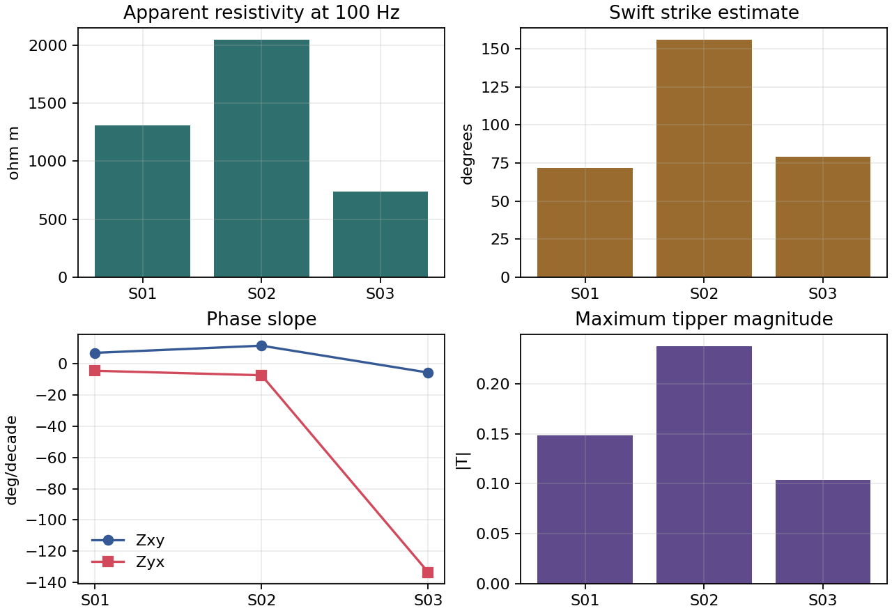
Computed diagnostics from the reproducible synthetic station set. The grid layout keeps resistivity, strike, phase-slope, and tipper checks visible together instead of separating them into unrelated figures.#
Read across the panels rather than ranking a station from one bar alone.
S02 has both the largest apparent resistivity and tipper amplitude, and
its 156-degree estimate is separated from the roughly 72–79 degree estimates
at S01 and S03. After reducing strike modulo 90 degrees, however,
S02 is near 66 degrees, so the apparent disagreement is modest. S03
is the clearest QC target because only its Zyx phase slope departs sharply;
that component-level anomaly should be inspected before any station-wide
rejection.
13.7.9. APIFrame Output#
For collection inputs, pass api=True when the result should carry pyCSAMT
API metadata in addition to tabular values.
>>> strike = strike_estimate(sites, api=True)
>>> rho = res_at_freq(sites, 100.0, api=True)
>>> slopes = phase_slope(sites, (10.0, 1000.0), api=True)
>>> tipper = tipper_magnitude(sites, api=True)

>>> print(strike.kind)
site.compute.strike
>>> print(rho.kind)
site.compute.resistivity
>>> print(slopes.kind)
site.compute.phase_slope
>>> print(tipper.kind)
site.compute.tipper
This is useful when diagnostics are emitted by CLI commands, agents, or pipelines that preserve result provenance.
13.7.10. Quality-Control Workflow#
In a real survey, computed diagnostics usually sit between selection/editing and reporting. The workflow is deliberately ordinary: filter unusable rows, make missing values explicit when needed, compute station tables, and merge the results into one review table.
>>> strike = strike_estimate(sites, api=False)
>>> rho100 = res_at_freq(sites, 100.0, how="nearest", api=False)
>>> slopes = phase_slope(sites, band=(10.0, 1000.0), api=False)
>>> tipper = tipper_magnitude(sites, api=False)

>>> qc = (
...     strike
...     .merge(rho100, on="station", how="outer")
...     .merge(slopes, on="station", how="outer")
...     .merge(tipper, on="station", how="outer")
... )

>>> print(qc.round(3).to_string(index=False))
station method  theta_deg   res_xy   res_yx  f_used  slope_xy  slope_yx  mean  median   max
    S01  swift       72.0 1310.819  946.216   100.0     6.875    -4.584 0.142   0.142 0.148
    S02  swift      156.0 2048.154 1478.463   100.0    11.459    -7.448 0.227   0.227 0.238
    S03  swift       79.0  737.336  532.247   100.0    -5.730  -133.479 0.099   0.099 0.104
13.7.11. Common Mistakes#
- Using diagnostics as final interpretation
These functions are quick screening tools. Confirm important decisions with maps, pseudo-sections, tensor plots, and inversion sensitivity tests.
- Mixing frequency axes without checking
f_used In
nearestmode, different stations may use different native frequencies. Always inspectf_usedbefore comparing values.- Ignoring missing arrays
Missing Z or tipper data are reported as
NaNrather than raising hard failures. Filter or fill intentionally before trusting the table.- Over-reading phase slope
A large phase slope may indicate structure, noise, phase wrapping, or a bad frequency band. Use it as a prompt for inspection, not as a standalone classifier.
13.7.12. Next Pages#
Continue with:
Site Selection for selecting stations before diagnostics;
Site Editing for preparing tensors, frequencies, names, and coordinates;
Export And Reporting for writing diagnostic summaries into survey deliverables;
Impedance Tensor for the physical meaning of impedance, apparent resistivity, phase, and tensor components.