
11.2. Quality-Control Confidence Scoring#
pycsamt.emtools.qc turns transfer-function quality control
into tables and figures. It does two related jobs:
summarize station-level data quality, coverage, SNR, tipper presence, and phase-tensor skew;
compute confidence ratios from several finite, bounded scores so that stations and individual station-frequency samples can be ranked, plotted, masked, or down-weighted before inversion.
Full callable signatures live in the API reference.
This page explains the confidence-ratio formulation, the table
workflow, the plotting workflow, and how confidence values should be
read in practice. Every example below uses pyCSAMT’s bundled
AMT line, data/AMT/WILLY_DATA/L18PLT, since all 28 stations
there carry real impedance-error tensors – the ingredient several of
the component scores need.
11.2.1. Why QC Is More Than Coverage#
A station can be complete and still be questionable. frac_ok=1.0
only says that impedance rows are finite. It does not say that the
off-diagonal modes agree, that diagonal leakage is small, that phase is
smooth, that uncertainty is low, or that the station is coherent with
its neighbours.
The QC module therefore separates three ideas:
coverageAre the required transfer-function rows finite?
confidenceHow trustworthy is a station or a station-frequency cell after combining coverage, uncertainty, tensor-shape, phase, and spatial criteria?
flagsWhich simple thresholds does a station or frequency cell fail?
11.2.2. Load A Survey#
All QC functions accept the usual pyCSAMT inputs, but a reproducible
script should normalize once with ensure_sites.
>>> from pathlib import Path
>>> from pycsamt.emtools import ensure_sites
>>> survey = ensure_sites(
...     Path("data/AMT/WILLY_DATA/L18PLT"),
...     recursive=True,
...     on_dup="replace",
...     strict=True,
...     verbose=1,
... )
Use strict=True for reports and automated processing. Use
strict=False in exploratory notebooks if you want empty plots to
render as “no data” messages.
11.2.3. The Confidence Ratio#
The composite confidence ratio is a weighted mean of available component scores:
Missing scores are ignored. Finite scores are clipped to [0, 1].
The default weights are:
Score |
Weight |
Meaning |
|---|---|---|
|
|
Finite impedance rows or components. |
|
|
Median relative impedance error. |
|
|
Similarity of |
|
|
Penalty for diagonal leakage into off-diagonal response. |
|
|
Penalty for abrupt off-diagonal phase jumps. |
|
|
Coherence with neighbouring stations. |
Except for coverage, each component reduces the tensor to a non-negative discrepancy \(m_k\), compares it with a positive tolerance \(\tau_k\), and maps the result to a bounded trust score:
A statistic of 0 scores a perfect 1; as \(m_k\) grows toward
\(\tau_k\) the score decays linearly to 0 and stays there beyond
it, so nothing is ever penalized twice or rewarded for being
implausibly clean. The coverage score is computed directly. For station
\(i\) with \(N_i\) frequencies and impedance tensor
\(Z_{i,f,ab}\), it is
whereas a frequency cell uses the fraction of its four finite tensor components. Thus station presence is deliberately strict: a row counts only when the complete impedance tensor is finite.
The remaining discrepancies used in (2) are
Their tolerances are respectively relerr_threshold=0.20,
offdiag_tolerance_log10=0.35, diagonal_leakage_max=0.35, and
phase_jump_tolerance_deg=90. At the frequency level, the first three
statistics are evaluated on one row. The phase score uses the strongest
adjacent jump touching that row for each off-diagonal mode, followed by
the median across the available modes. The small \(\epsilon\)
prevents division by zero and is numerical, not a tunable tolerance.
Spatial coherence first forms the log-response proxy
At station level \(r_i={\rm med}_f(r_{i,f})\); at frequency level \(r_{i,f}\) is retained. The spatial discrepancy is
where \(\mathcal N_i\) contains the immediately adjacent available stations. The omitted physical constants cancel in this relative logarithmic comparison; \(r\) should therefore be read as a resistivity-like proxy, not a reported apparent resistivity.
At station level the discrepancies summarize the frequency axis, which
is why station_confidence_table returns one score per station. At
frequency level the analogous local quantities are evaluated row by
row. Consequently, a coherent station aggregate can still contain weak
individual frequencies.
The default confidence bands are:
CR >= 0.95: safe under the default policy;0.85 <= CR < 0.95: marginal or recoverable;CR < 0.85: high-priority review or down-weighting candidate.
Important
These are operational defaults, not universal geophysical laws. A low score can reflect genuine dimensionality or a sharp geological boundary. Inspect the component scores and response curves before deleting data.
11.2.4. Compute A Confidence Ratio Directly#
Use confidence_ratio when you already have scores and want to apply
the same weighted formula used by the tables.
>>> from pycsamt.emtools.qc import confidence_ratio
>>> scores = {
...     "coverage": 1.00,
...     "uncertainty": 0.82,
...     "offdiag": 0.76,
...     "diagonal": 0.55,
...     "phase": 0.90,
...     "spatial": 0.88,
... }
>>> cr, cr_err = confidence_ratio(scores, n_freq=53, return_error=True)
>>> print(f"CR={cr:.3f} +/- {cr_err:.3f}")
CR=0.861 +/- 0.141
confidence_err is not a formal statistical uncertainty on
\(\mathrm{CR}\) – it is a cheap, honest stand-in for one:
With six components on hand, as in the example above,
\(\sigma_{\mathrm{CR}}\) is simply the population standard deviation
of {1.00, 0.82, 0.76, 0.55, 0.90, 0.88}, which is exactly the
0.141 printed above – the components disagree with each other, and
that disagreement is the reported uncertainty. When only one
component survives (most often coverage alone, when no error tensor
or neighbouring station exists to score against), there is nothing to
disagree with, so the formula falls back to the binomial-style standard
error \(\sqrt{\mathrm{CR}(1-\mathrm{CR})/n_{\mathrm{freq}}}\) instead.
11.2.5. Station QC Summary#
build_qc_table is the first station-level table. It reports the
number of frequencies, finite-row coverage, tipper availability, median
row SNR when z_err exists, period range, and optional
phase-tensor skew.
>>> from pycsamt.emtools import build_qc_table, ensure_sites
>>> survey = ensure_sites("data/AMT/WILLY_DATA/L18PLT", strict=True)
>>> qc = build_qc_table(survey, include_skew=True, api=False)
>>> qc[["station", "n_freq", "n_ok", "frac_ok", "n_tip", "snr_med", "pmin", "pmax", "skew_med"]].head()
   station  n_freq  n_ok  frac_ok  ...    snr_med      pmin      pmax   skew_med
0  18-001A      53    53      1.0  ...  17.658396  0.000096  0.992063   4.809977
1  18-002U      53    53      1.0  ...  16.687366  0.000096  0.992063   6.596544
2  18-003A      53    53      1.0  ...  12.031672  0.000096  0.992063  11.018588
3  18-004A      53    53      1.0  ...  10.430580  0.000096  0.992063  14.509282
4  18-005U      53    53      1.0  ...  14.360341  0.000096  0.992063   9.171151

[5 rows x 9 columns]
Read frac_ok as completeness, not as full confidence. Read
snr_med as a row-level signal-to-error ratio when impedance error
tensors are available. Read skew_med as structural/tensor
complexity, not automatically as bad acquisition – it is the median
absolute phase tensor asymmetry angle \(|\beta|\) across a
station’s frequencies, the same quantity the skew glossary
entry defines.
11.2.6. Station Flags#
qc_flags adds simple threshold labels to the station QC table.
>>> from pycsamt.emtools import qc_flags
>>> flags = qc_flags(
...     "data/AMT/WILLY_DATA/L18PLT",
...     min_frac_ok=0.60,
...     min_snr_med=2.0,
...     max_skew_med=6.0,
... )
>>> flagged = flags[flags["flags"] != ""]
>>> print(len(flagged), "of", len(flags), "stations flagged")
27 of 28 stations flagged
>>> flagged[["station", "frac_ok", "snr_med", "skew_med", "flags"]].head()
   station  frac_ok    snr_med   skew_med      flags
1  18-002U      1.0  16.687366   6.596544  high_skew
2  18-003A      1.0  12.031672  11.018588  high_skew
3  18-004A      1.0  10.430580  14.509282  high_skew
4  18-005U      1.0  14.360341   9.171151  high_skew
5  18-006A      1.0  13.272516  12.375357  high_skew
Every station is fully covered (frac_ok=1.0 throughout) and every
station’s median row SNR clears min_snr_med=2.0 by a wide margin, so
high_skew is the only flag this survey ever raises, and it raises it
for all but one station: only 18-001A (skew_med=4.81) falls
under the default max_skew_med=6.0 threshold, while the rest run
from 6.60 up past 50 degrees. That is not a data defect – it is
a genuinely 2-D/3-D structural line, expressed through a threshold tuned
for near-1-D settings. Possible station flags include low_coverage,
low_snr, and high_skew. A high-skew flag can be a real
structural signal. It does not mean the station should automatically be
deleted.
11.2.7. Presence Confidence Versus Composite Confidence#
station_confidence_table has two modes. method="presence" is
coverage-only. method="composite" combines all available component
scores.
>>> from pycsamt.emtools import station_confidence_table
>>> presence = station_confidence_table(
...     "data/AMT/WILLY_DATA/L18PLT",
...     method="presence",
...     api=False,
... )
>>> composite = station_confidence_table(
...     "data/AMT/WILLY_DATA/L18PLT",
...     method="composite",
...     api=False,
... )
>>> print("presence range", presence["confidence"].min(), presence["confidence"].max())
presence range 1.0 1.0
>>> print("composite range", composite["confidence"].min(), composite["confidence"].max())
composite range 0.5440199944767435 0.8119223880398303
>>> ranked = composite.sort_values("confidence")
>>> ranked[["station", "confidence", "coverage", "uncertainty", "offdiag", "diagonal", "phase", "spatial"]].head()
    station  confidence  coverage  ...  diagonal     phase   spatial
22  18-022U    0.544020       1.0  ...  0.000000  0.941638  0.000000
21  18-021B    0.574114       1.0  ...  0.000000  0.937891  0.232771
17  18-018A    0.578410       1.0  ...  0.086979  0.957546  0.000000
20  18-021U    0.594344       1.0  ...  0.000000  0.938165  0.233576
16  18-017U    0.595479       1.0  ...  0.261699  0.969783  0.038160

[5 rows x 8 columns]
Presence confidence is a flat 1.0 everywhere – every row is
finite, so a coverage-only view has nothing left to say about this
particular survey. Composite confidence spreads from
\(\approx 0.54\) to \(\approx 0.81\) instead: the coverage-only
view was hiding real, measurable quality variation. If presence
confidence is high everywhere but composite confidence varies, the
survey is complete but not equally trustworthy everywhere. That is
common in real EM data.
11.2.8. Customize Confidence Weights#
Use custom weights when a project has a clear processing policy. For example, inversion preparation may emphasize uncertainty and coverage, while structural interpretation may care more about off-diagonal and spatial coherence.
>>> weights = {
...     "coverage": 0.40,
...     "uncertainty": 0.30,
...     "offdiag": 0.10,
...     "diagonal": 0.05,
...     "phase": 0.05,
...     "spatial": 0.10,
... }
>>> table = station_confidence_table(
...     "data/AMT/WILLY_DATA/L18PLT",
...     method="composite",
...     weights=weights,
...     relerr_threshold=0.25,
...     offdiag_tolerance_log10=0.40,
...     diagonal_leakage_max=0.40,
...     phase_jump_tolerance_deg=90.0,
...     spatial_tolerance_log10=0.60,
...     api=False,
... )
>>> table.sort_values("confidence")[["station", "distance_m", "confidence", "coverage", "uncertainty", "offdiag", "diagonal", "phase", "spatial"]].head()
    station  distance_m  confidence  ...  diagonal     phase   spatial
22  18-022U      4400.0    0.630495  ...  0.000000  0.941638  0.000000
21  18-021B      4200.0    0.658344  ...  0.000000  0.937891  0.232771
17  18-018A      3400.0    0.666682  ...  0.201107  0.957546  0.000000
16  18-017U      3200.0    0.672222  ...  0.353986  0.969783  0.038160
20  18-021U      4000.0    0.682870  ...  0.000000  0.938165  0.233576

[5 rows x 9 columns]
The worst station is still 18-022U under either weighting – its
penalty is concentrated enough (zero diagonal and near-zero
spatial) that it stays worst regardless of emphasis. Changing
thresholds changes the meaning of the scores. Record custom weights and
thresholds in reports so another user can reproduce your confidence
classes.
11.2.9. Frequency-Level Confidence#
frequency_confidence_table returns one row per station-frequency
sample, scored with the same six formulas and the same
\(\mathrm{CR}_{i,f}\) weighting as the station table above – the
only change is that each \(m_k\) is now evaluated at a single
frequency rather than medianed across the whole station. This is the
table to use for period-band decisions, masks, and inversion
down-weighting.
>>> from pycsamt.emtools import frequency_confidence_table
>>> freq_qc = frequency_confidence_table(
...     "data/AMT/WILLY_DATA/L18PLT",
...     method="composite",
...     ci_hi=0.95,
...     ci_lo=0.85,
...     api=False,
... )
>>> freq_qc.columns.tolist()
['station', 'station_index', 'distance_m', 'frequency_hz', 'period_s', 'log10_period', 'confidence', 'confidence_err', 'method', 'n_components', 'coverage', 'uncertainty', 'offdiag', 'diagonal', 'phase', 'spatial', 'logrho_proxy', 'flags']
>>> freq_qc[["station", "frequency_hz", "period_s", "confidence", "flags"]].head()
   station  ...                                              flags
0  18-001A  ...  recoverable,high_error,offdiag_mismatch,diagon...
1  18-001A  ...  reject,high_error,offdiag_mismatch,diagonal_le...
2  18-001A  ...  reject,high_error,offdiag_mismatch,diagonal_le...
3  18-001A  ...  reject,high_error,offdiag_mismatch,diagonal_le...
4  18-001A  ...  reject,high_error,offdiag_mismatch,diagonal_le...

[5 rows x 5 columns]
>>> rejected = freq_qc[freq_qc["flags"].str.contains("reject", na=False)]
>>> print("rejected cells:", len(rejected), "of", len(freq_qc))
rejected cells: 1479 of 1484
Frequency flags can include reject, recoverable, missing,
high_error, offdiag_mismatch, diagonal_leakage,
phase_jump, and spatial_outlier. Nearly every one of this
survey’s 1484 station-frequency cells reads reject at the frequency
level. The station-level composite range of 0.54–0.81 is also below
the default 0.85 boundary, but aggregation makes the station scores less
extreme than many individual cells. Use the frequency table when the
decision concerns a period band rather than a complete station.
11.2.10. Build A Mask From Confidence#
The QC module does not force one masking policy. You can build one from the confidence table.
>>> table = frequency_confidence_table(
...     "data/AMT/WILLY_DATA/L18PLT",
...     method="composite",
...     ci_lo=0.85,
...     api=False,
... )
>>> keep = table["confidence"] >= 0.85
>>> review = (table["confidence"] >= 0.70) & (table["confidence"] < 0.85)
>>> drop = table["confidence"] < 0.70
>>> print("keep:", int(keep.sum()))
keep: 5
>>> print("review:", int(review.sum()))
review: 533
>>> print("drop:", int(drop.sum()))
drop: 946
Use a review band instead of a hard delete when the flagged frequencies line up with known structural complexity. Low confidence is a prompt for inspection, not always proof of bad data.
11.2.11. Survey-Scale Confidence Views#
The L18 examples above explain one profile. Spatial confidence figures
need more than one non-collinear line, so the examples in this section
use all five WILLY_DATA profiles (128 stations). Line membership is
derived from the station prefix only for display; it does not alter the
confidence calculation.
>>> from pycsamt.emtools import ensure_sites, station_confidence_table
>>> all_lines = ensure_sites("data/AMT/WILLY_DATA", recursive=True)
>>> all_table = station_confidence_table(
...     all_lines, method="composite", api=False,
... )
>>> line_labels = {
...     str(station): f"L{str(station).split('-', 1)[0]}"
...     for station in all_table["station"]
... }
>>> len(all_table), sorted(set(line_labels.values()))
(128, ['L18', 'L22', 'L26', 'L30', 'L34'])
The complete, executable figure-generation script is available below. It writes every image in this section and exports the confidence surface as CSV and Surfer DSAA grid files.
Generate all survey-scale confidence figuresClick to inspect and copy the complete code
  1#!/usr/bin/env python
  2# Author: LKouadio <etanoyau@gmail.com>
  3# License: LGPL-3.0
  4"""Generate confidence figures for the EMTools QC user guide.
  5
  6Run from the repository root::
  7
  8    python docs/scripts/generate_user_guide_emtools_qc_confidence_figures.py \
  9        --save-dir docs/source/images/user_guide/emtools/confidence
 10
 11Use ``--save-dir DIR`` to save both figures instead of opening them.
 12The single-line example uses L18PLT. The contour example uses all five
 13WILLY_DATA profiles, because interpolation from one line is not a valid
 14two-dimensional confidence map.
 15"""
 16
 17from __future__ import annotations
 18
 19import argparse
 20from pathlib import Path
 21
 22import matplotlib.pyplot as plt
 23
 24from pycsamt.emtools import (
 25    ensure_sites,
 26    export_confidence_map,
 27    plot_confidence_before_after,
 28    plot_confidence_component_map,
 29    plot_confidence_coverage_curve,
 30    plot_confidence_distribution,
 31    plot_confidence_grid_map,
 32    plot_confidence_heatmap,
 33    plot_confidence_map,
 34    plot_confidence_method_comparison,
 35    plot_confidence_rank,
 36    plot_confidence_risk_map,
 37    station_confidence_table,
 38)
 39
 40
 41def _repository_root() -> Path:
 42    return Path(__file__).resolve().parents[2]
 43
 44
 45def _line_labels(sites) -> dict[str, str]:
 46    table = station_confidence_table(sites, method="composite", api=False)
 47    return {
 48        str(station): f"L{str(station).split('-', 1)[0]}"
 49        for station in table["station"]
 50    }
 51
 52
 53def make_figures():
 54    """Return route, filled-contour, and labelled-isoline map axes."""
 55    data_root = _repository_root() / "data" / "AMT" / "WILLY_DATA"
 56    line18 = data_root / "L18PLT"
 57
 58    route_ax = plot_confidence_map(
 59        line18,
 60        method="composite",
 61        mode="route",
 62        station_labels=True,
 63        station_label_step=4,
 64        show_confidence_values=True,
 65        confidence_value_step=2,
 66        confidence_value_fmt="{:.2f}",
 67        confidence_value_fontsize=6.5,
 68        recursive=False,
 69    )
 70    route_ax.set_title("L18 confidence along the surveyed route")
 71
 72    all_lines = ensure_sites(data_root, recursive=True)
 73    contour_ax = plot_confidence_map(
 74        all_lines,
 75        method="composite",
 76        mode="contour",
 77        line_labels=_line_labels(all_lines),
 78        boundary_levels=[0.50, 0.85, 0.90, 1.00],
 79        show_contour_lines=False,
 80        show_threshold_contours=True,
 81        threshold_linewidth=1.6,
 82    )
 83    contour_ax.set_title("WILLY_DATA confidence map — boundary contours only")
 84
 85    line_ax = plot_confidence_map(
 86        all_lines,
 87        method="composite",
 88        mode="contour",
 89        line_labels=_line_labels(all_lines),
 90        show_contour_lines=True,
 91        contour_line_levels=[0.55, 0.60, 0.65, 0.70, 0.75, 0.80],
 92        contour_line_colors="#303030",
 93        contour_linewidths=0.8,
 94        contour_linestyles="solid",
 95        contour_labels=True,
 96        contour_label_fmt="%.2f",
 97        contour_label_fontsize=6.5,
 98        threshold_line_color="black",
 99        threshold_linewidth=1.6,
100        threshold_linestyle="--",
101    )
102    line_ax.set_title("WILLY_DATA confidence contours with labelled isolines")
103    return route_ax, contour_ax, line_ax
104
105
106def main() -> None:
107    parser = argparse.ArgumentParser(description=__doc__)
108    parser.add_argument("--save-dir", type=Path)
109    parser.add_argument(
110        "--export-dir",
111        type=Path,
112        help="Write station CSV and Surfer DSAA confidence grid.",
113    )
114    args = parser.parse_args()
115    axes = make_figures()
116    data_root = _repository_root() / "data" / "AMT" / "WILLY_DATA"
117    all_lines = ensure_sites(data_root, recursive=True)
118    component_fig = plot_confidence_component_map(
119        all_lines,
120        method="composite",
121        line_labels=_line_labels(all_lines),
122        ncols=4,
123        marker_size=32.0,
124    )
125    comparison_fig = plot_confidence_method_comparison(
126        all_lines,
127        line_labels=_line_labels(all_lines),
128        marker_size=34.0,
129        map_aspect="auto",
130    )
131    risk_ax = plot_confidence_risk_map(
132        all_lines,
133        method="composite",
134        line_labels=_line_labels(all_lines),
135        mode="contour",
136        risk_levels=[0.0, 0.05, 0.10, 0.15, 0.25, 0.35, 0.50, 0.75, 1.0],
137        station_labels=False,
138        map_aspect="auto",
139    )
140    heatmap_ax = plot_confidence_heatmap(
141        all_lines,
142        method="composite",
143        line_labels=_line_labels(all_lines),
144        station_order="route",
145        annotate=False,
146        station_label_step=4,
147    )
148    distribution_fig = plot_confidence_distribution(
149        all_lines,
150        method="both",
151        line_labels=_line_labels(all_lines),
152        bins=18,
153    )
154    rank_fig = plot_confidence_rank(
155        all_lines,
156        method="composite",
157        line_labels=_line_labels(all_lines),
158        order="worst",
159        annotate_stations=False,
160        show_iqr=True,
161    )
162    grid_ax = plot_confidence_grid_map(
163        all_lines,
164        method="composite",
165        line_labels=_line_labels(all_lines),
166        grid_shape=(220, 180),
167        interpolation="linear",
168        show_grid_edges=False,
169        map_aspect="auto",
170    )
171    coverage_fig = plot_confidence_coverage_curve(
172        all_lines,
173        method="composite",
174        line_labels=_line_labels(all_lines),
175    )
176    before_after_fig = plot_confidence_before_after(
177        all_lines,
178        before_method="presence",
179        after_method="composite",
180        before_label="Presence",
181        after_label="Composite",
182        line_labels=_line_labels(all_lines),
183        show_station_labels=False,
184    )
185    if args.save_dir is None:
186        plt.show()
187        return
188    args.save_dir.mkdir(parents=True, exist_ok=True)
189    names = (
190        "confidence_route",
191        "confidence_contour",
192        "confidence_contour_lines",
193    )
194    for name, ax in zip(names, axes):
195        ax.figure.savefig(
196            args.save_dir / f"{name}.png",
197            dpi=180,
198            bbox_inches="tight",
199        )
200    component_fig.savefig(
201        args.save_dir / "confidence_component_map.png",
202        dpi=220,
203        bbox_inches="tight",
204    )
205    comparison_fig.savefig(
206        args.save_dir / "confidence_method_comparison.png",
207        dpi=220,
208        bbox_inches="tight",
209    )
210    risk_ax.figure.savefig(
211        args.save_dir / "confidence_risk_map.png",
212        dpi=220,
213        bbox_inches="tight",
214    )
215    heatmap_ax.figure.savefig(
216        args.save_dir / "confidence_heatmap.png",
217        dpi=220,
218        bbox_inches="tight",
219    )
220    distribution_fig.savefig(
221        args.save_dir / "confidence_distribution.png",
222        dpi=220,
223        bbox_inches="tight",
224    )
225    rank_fig.savefig(
226        args.save_dir / "confidence_rank.png",
227        dpi=220,
228        bbox_inches="tight",
229    )
230    grid_ax.figure.savefig(
231        args.save_dir / "confidence_grid_map.png",
232        dpi=220,
233        bbox_inches="tight",
234    )
235    coverage_fig.savefig(
236        args.save_dir / "confidence_coverage_curve.png",
237        dpi=220,
238        bbox_inches="tight",
239    )
240    before_after_fig.savefig(
241        args.save_dir / "confidence_before_after.png",
242        dpi=220,
243        bbox_inches="tight",
244    )
245    if args.export_dir is not None:
246        args.export_dir.mkdir(parents=True, exist_ok=True)
247        export_confidence_map(
248            all_lines,
249            method="composite",
250            line_labels=_line_labels(all_lines),
251            csv_path=args.export_dir / "confidence_map.csv",
252            surfer_path=args.export_dir / "confidence_map.grd",
253            grid_shape=(200, 200),
254        )
255
256
257if __name__ == "__main__":
258    main()
11.2.11.1. Route, contour, and regular-grid maps#
plot_confidence_map uses measured longitude/latitude when available
and otherwise falls back to easting/northing. Route mode orders stations
from coordinate-derived chainage; it does not trust lexical station names.
Contour mode requires at least three non-collinear locations and is
restricted to the triangulated survey footprint.
>>> from pycsamt.emtools import plot_confidence_map
>>> route_ax = plot_confidence_map(
...     "data/AMT/WILLY_DATA/L18PLT",
...     method="composite",
...     mode="route",
...     show_confidence_values=True,
...     confidence_value_step=2,
... )
>>> contour_ax = plot_confidence_map(
...     all_lines,
...     method="composite",
...     mode="contour",
...     line_labels=line_labels,
...     boundary_levels=[0.50, 0.85, 0.90, 1.00],
...     show_contour_lines=False,
...     show_threshold_contours=True,
... )
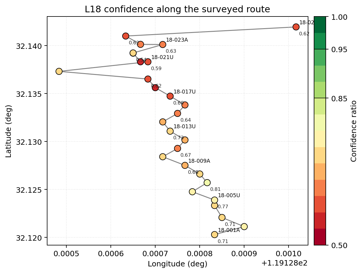
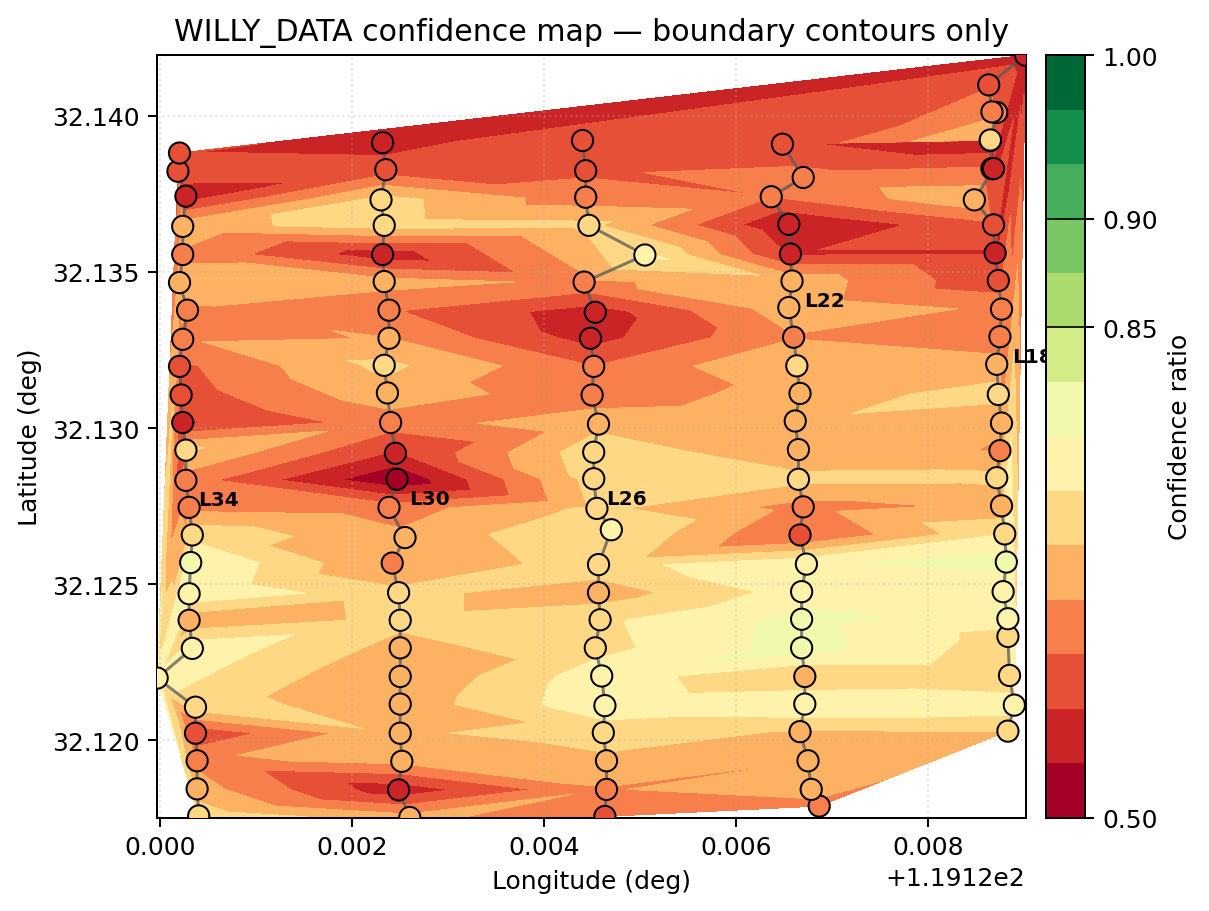
The route view reveals station-scale variability without implying two-dimensional coverage. The multi-line contour is appropriate for a spatial overview, but no 0.85, 0.90, or 1.00 isoline appears in this dataset because the observed composite maximum is about 0.81. Omitting an absent boundary is the scientifically correct result.
Ordinary labelled isolines can be added independently of the decision
boundaries. plot_confidence_grid_map instead evaluates the same
triangulated field on a regular \(n_x\times n_y\) grid. Its masked
cells outside the convex hull remain blank and its arrays are available
as ax._pycsamt_grid_x, ax._pycsamt_grid_y, and
ax._pycsamt_confidence_grid.
>>> from pycsamt.emtools import plot_confidence_grid_map
>>> isoline_ax = plot_confidence_map(
...     all_lines,
...     mode="contour",
...     line_labels=line_labels,
...     show_contour_lines=True,
...     contour_line_levels=[0.55, 0.60, 0.65, 0.70, 0.75, 0.80],
...     contour_line_colors="0.2",
...     contour_labels=True,
... )
>>> grid_ax = plot_confidence_grid_map(
...     all_lines,
...     line_labels=line_labels,
...     grid_shape=(220, 180),
...     interpolation="linear",
... )
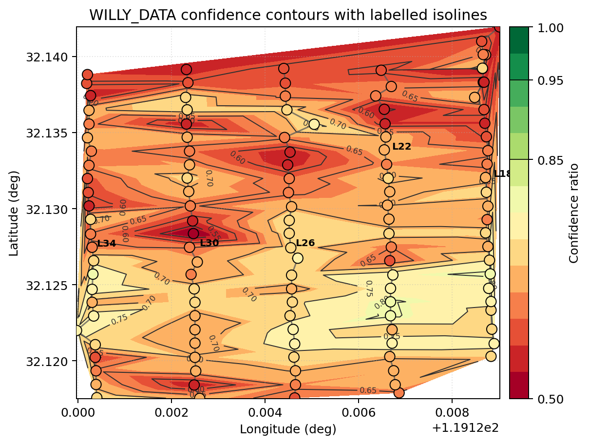
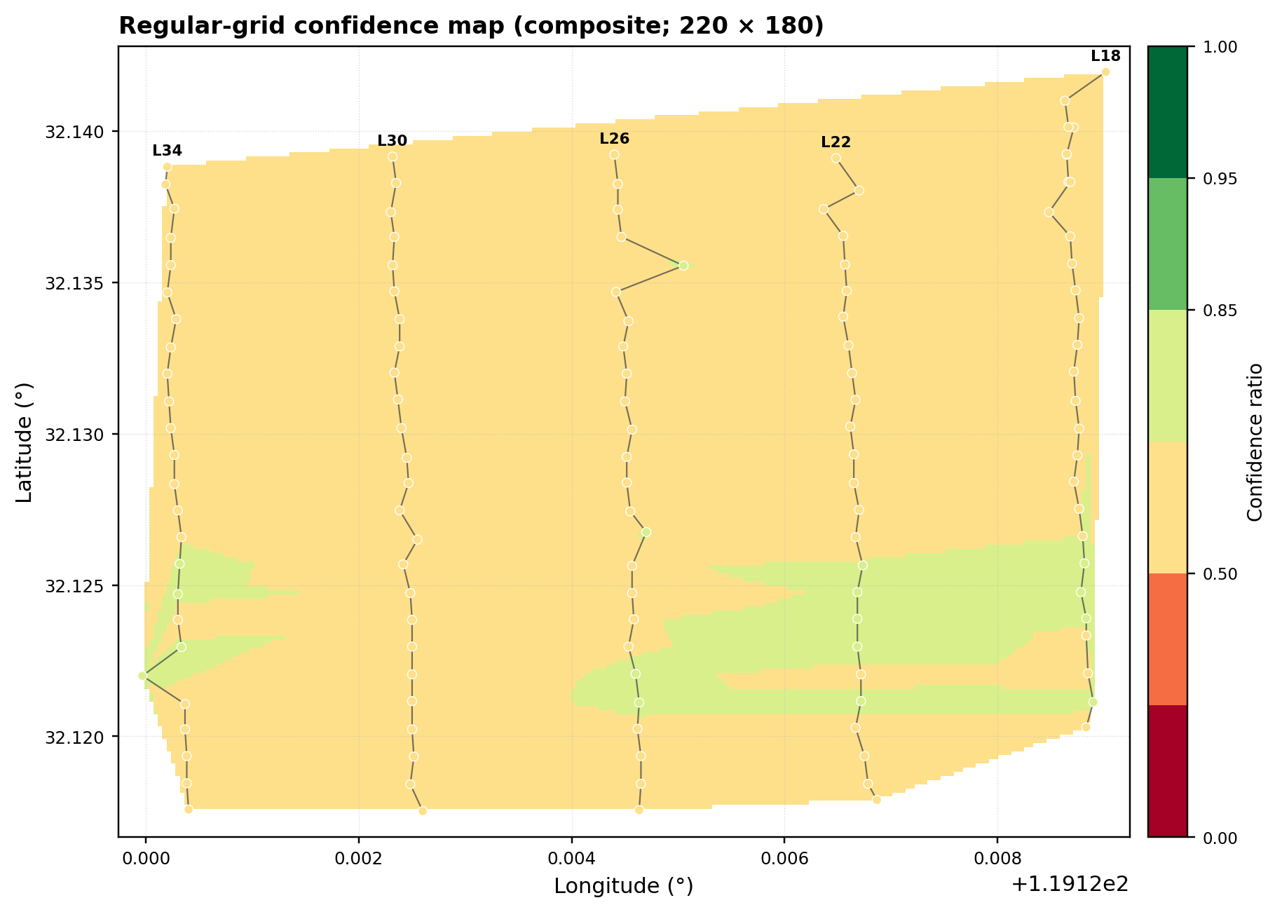
The stepped edges in the regular-grid figure are raster-cell boundaries,
not geological discontinuities. Use max_triangle_edge to suppress
triangles spanning an unjustified gap between lines. interpolation
may be "linear" or "cubic"; cubic interpolation is visually
smoother but should not be interpreted as new measurements.
For external mapping, export_confidence_map writes station values and
the regular field without coupling export to plotting:
>>> from pycsamt.emtools import export_confidence_map
>>> outputs = export_confidence_map(
...     all_lines,
...     method="composite",
...     line_labels=line_labels,
...     csv_path="confidence_map.csv",
...     surfer_path="confidence_map.grd",
...     grid_shape=(200, 200),
... )
>>> sorted(outputs)
['csv', 'surfer']
The Surfer file uses ASCII DSAA format. As with the plotted grid, cells outside the convex hull are blank. Export CSV instead of a grid for a single collinear profile.
11.2.11.2. Diagnosing which component controls confidence#
plot_confidence_component_map applies one fixed 0–1 scale to the
overall score and all six terms in (1).
This fixed normalization is essential: independently rescaling each
panel would make a weak component look artificially strong.
>>> from pycsamt.emtools import plot_confidence_component_map
>>> component_fig = plot_confidence_component_map(
...     all_lines,
...     method="composite",
...     line_labels=line_labels,
...     ncols=4,
...     marker_size=32,
... )
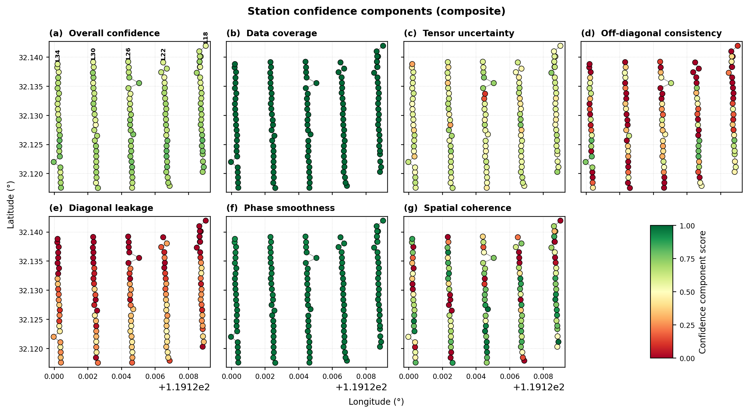
Overall confidence and the six component scores on shared coordinates.#
Coverage and phase smoothness are consistently strong in WILLY_DATA, whereas diagonal leakage, off-diagonal consistency, and spatial coherence contain repeated low-score stations. The overall composite therefore remains below the safe threshold even though the transfer functions are complete. This is precisely the distinction between presence and trustworthiness introduced above.
plot_confidence_heatmap presents the same decomposition as a compact
station-by-component matrix. Gray cells mean that a component could not
be evaluated; they do not mean zero confidence.
>>> from pycsamt.emtools import plot_confidence_heatmap
>>> heatmap_ax = plot_confidence_heatmap(
...     all_lines,
...     method="composite",
...     line_labels=line_labels,
...     station_order="route",
...     annotate=False,
...     station_label_step=4,
... )
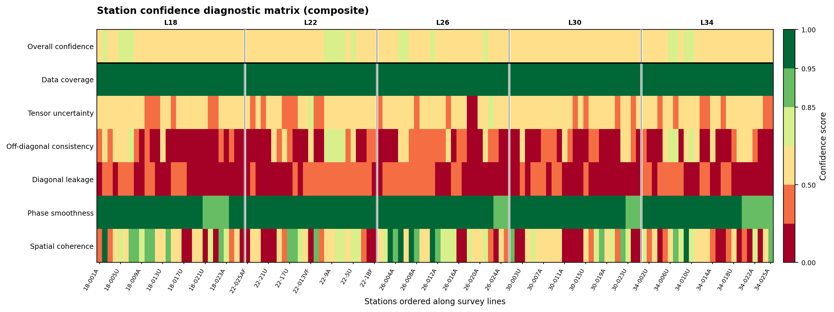
Confidence diagnostic matrix with stations grouped by survey line.#
The dark-green coverage row confirms complete input, while coherent red blocks in the tensor-shape and spatial rows identify systematic rather than isolated penalties. Use cell annotations for small surveys; for 128 stations, thinning labels and suppressing values preserves the pattern.
11.2.11.3. Comparing methods and processing states#
plot_confidence_method_comparison matches station coordinates and
shows presence, composite, and their difference
\(\Delta\mathrm{CR}=\mathrm{CR}_{\rm composite}-
\mathrm{CR}_{\rm presence}\). The first two panels share 0–1 limits;
the difference panel is symmetric about zero.
>>> from pycsamt.emtools import plot_confidence_method_comparison
>>> comparison_fig = plot_confidence_method_comparison(
...     all_lines,
...     line_labels=line_labels,
...     marker_size=34,
... )
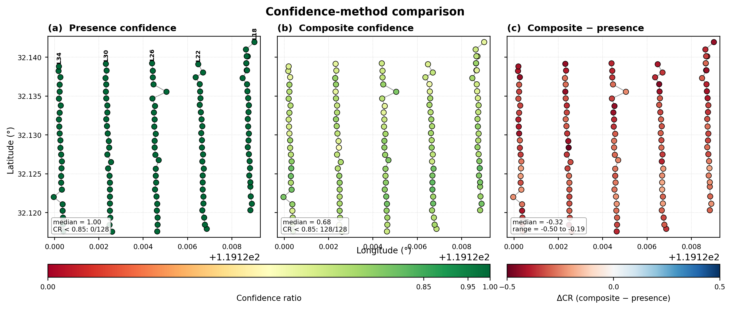
Presence, composite, and paired method difference at 128 stations.#
Presence is 1.0 throughout because every impedance row is finite. Composite confidence is lower by about 0.19–0.50 because it includes the additional discrepancies in (4). This difference is not a processing loss; it is information that the presence method does not attempt to represent.
For genuine processing audits, pass separate datasets to
plot_confidence_before_after. For matched station \(i\), the
reported change is
Values larger than change_tolerance are improvements, values below
its negative are degradations, and smaller absolute changes are stable.
The default tolerance is 0.01.
>>> from pycsamt.emtools import plot_confidence_before_after
>>> audit_fig = plot_confidence_before_after(
...     all_lines,
...     before_method="presence",
...     after_method="composite",
...     before_label="Presence",
...     after_label="Composite",
...     line_labels=line_labels,
...     show_station_labels=False,
... )
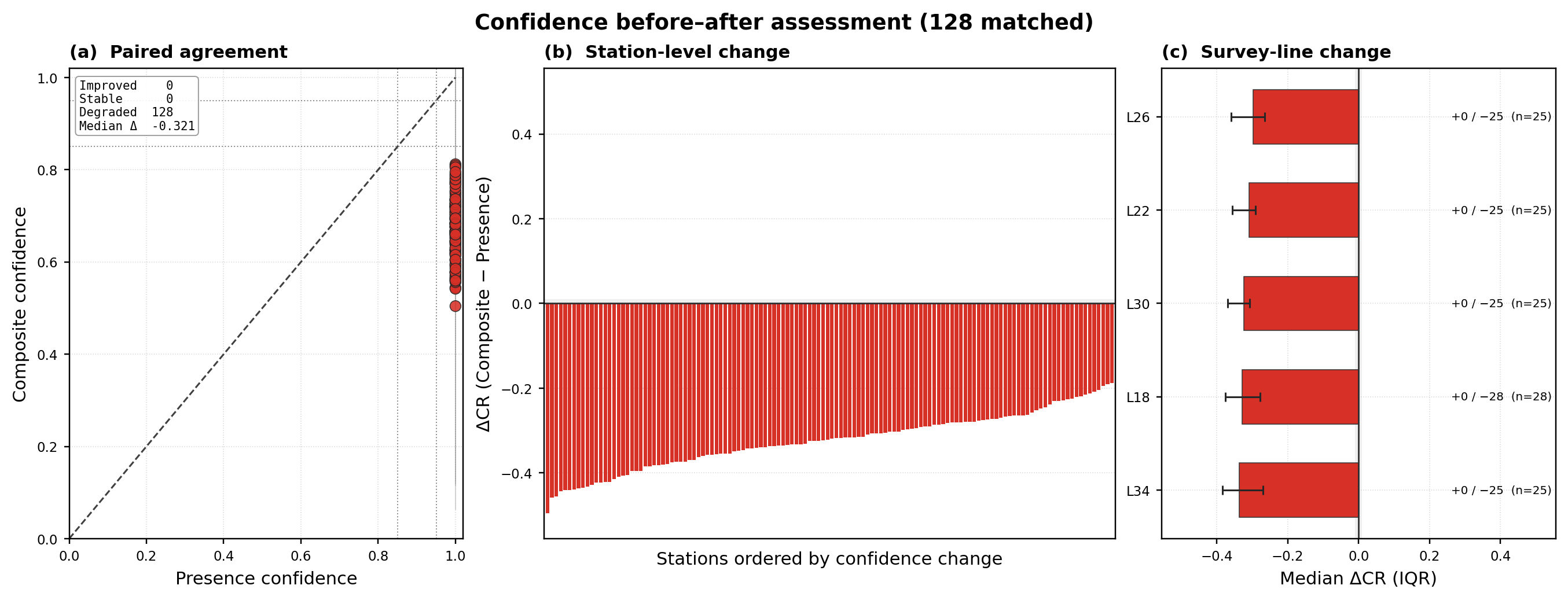
Paired scoring audit, ordered station changes, and line-level median change.#
This reproducible example audits two scoring methods on one dataset, so
all changes are negative by construction. In a processing workflow,
replace the first argument with the unprocessed survey and pass the
processed survey as after_sites while keeping both methods
"composite". Unmatched station names are retained on the returned
figure for auditability and excluded from paired statistics.
11.2.11.4. Risk, distributions, and priorities#
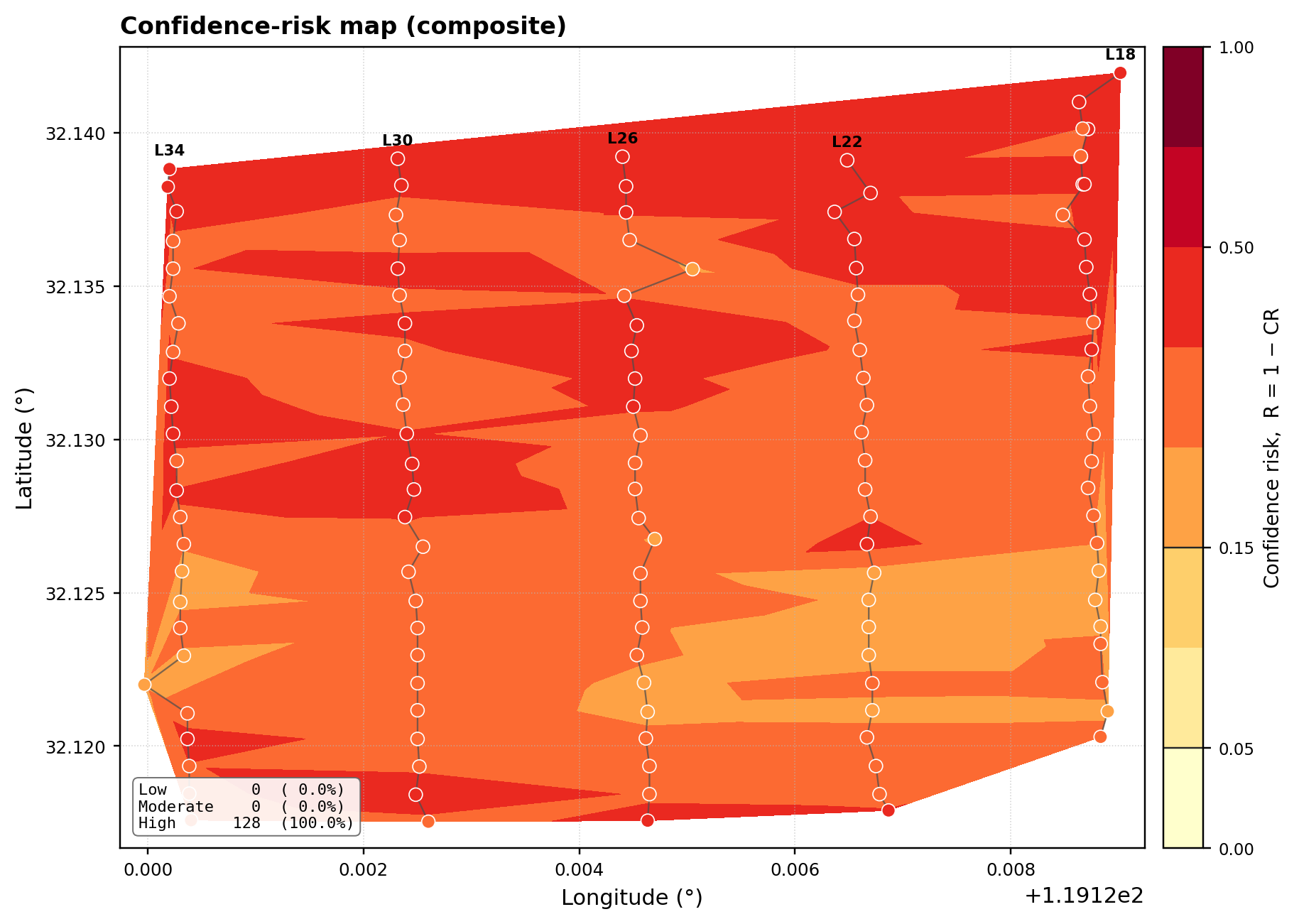
Confidence risk is the complement of confidence,
Consequently, the default CR limits 0.95 and 0.85 correspond to risk
limits 0.05 and 0.15. plot_confidence_risk_map reports low,
moderate, and high-risk station counts and does not invent a new quality
metric.
>>> from pycsamt.emtools import plot_confidence_risk_map
>>> risk_ax = plot_confidence_risk_map(
...     all_lines,
...     line_labels=line_labels,
...     mode="contour",
... )
Complementary confidence risk across WILLY_DATA.#
All 128 composite scores are below 0.85, so every station belongs to the default high-risk review class. The orange-to-red variation still ranks relative risk within that class; it must not be read as evidence that the interpolated space between lines was directly measured.
plot_confidence_distribution combines density, empirical cumulative
fraction, and line-wise violin summaries. The empirical curve is exact;
the Gaussian density is a visualization whose bandwidth does not change
the underlying station scores.
>>> from pycsamt.emtools import plot_confidence_distribution
>>> distribution_fig = plot_confidence_distribution(
...     all_lines,
...     method="both",
...     line_labels=line_labels,
...     bins=18,
... )
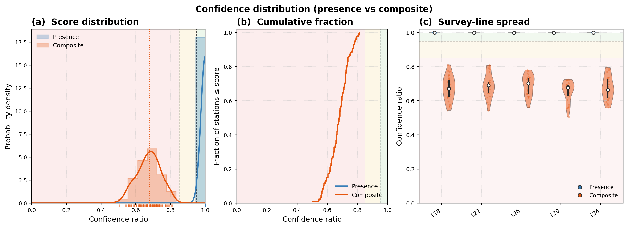
Presence/composite density, cumulative fraction, and survey-line spread.#
The spike at presence CR = 1.0 and the broad composite mode near 0.6–0.75 summarize the method difference compactly. The line violins show that the composite spread is not controlled by a single profile.
plot_confidence_rank turns the same values into an operational
priority list. Station rank is exact; the line panel uses the median and
interquartile range by default so an isolated extreme station does not
control an entire line’s rank.
>>> from pycsamt.emtools import plot_confidence_rank
>>> rank_fig = plot_confidence_rank(
...     all_lines,
...     method="composite",
...     line_labels=line_labels,
...     order="worst",
...     annotate_stations=False,
... )
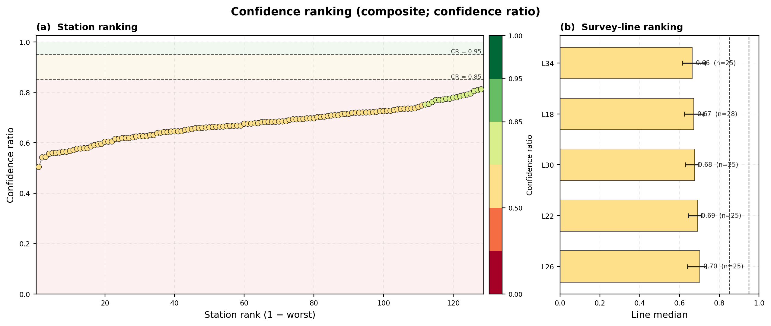
Worst-first station priorities and robust survey-line ranking.#
The WILLY station curve rises from about 0.50 to 0.81. L34 has the lowest line median and L26 the highest in this run, but their overlapping IQRs caution against treating that ordering as a sharp statistical separation.
11.2.11.5. Coverage retained as a threshold rises#
plot_confidence_coverage_curve asks an operational question: how
much survey remains when the minimum accepted CR is \(t\)? The
station and valid-data retention functions are
Connected-route retention sums only station-to-station segment lengths whose two endpoints meet the threshold, divided by total route length. It can therefore fall faster than station retention when accepted stations become spatially fragmented. The reported AUC is \(\int_0^1 C(t)\,dt\).
>>> from pycsamt.emtools import plot_confidence_coverage_curve
>>> coverage_fig = plot_confidence_coverage_curve(
...     all_lines,
...     method="composite",
...     line_labels=line_labels,
... )
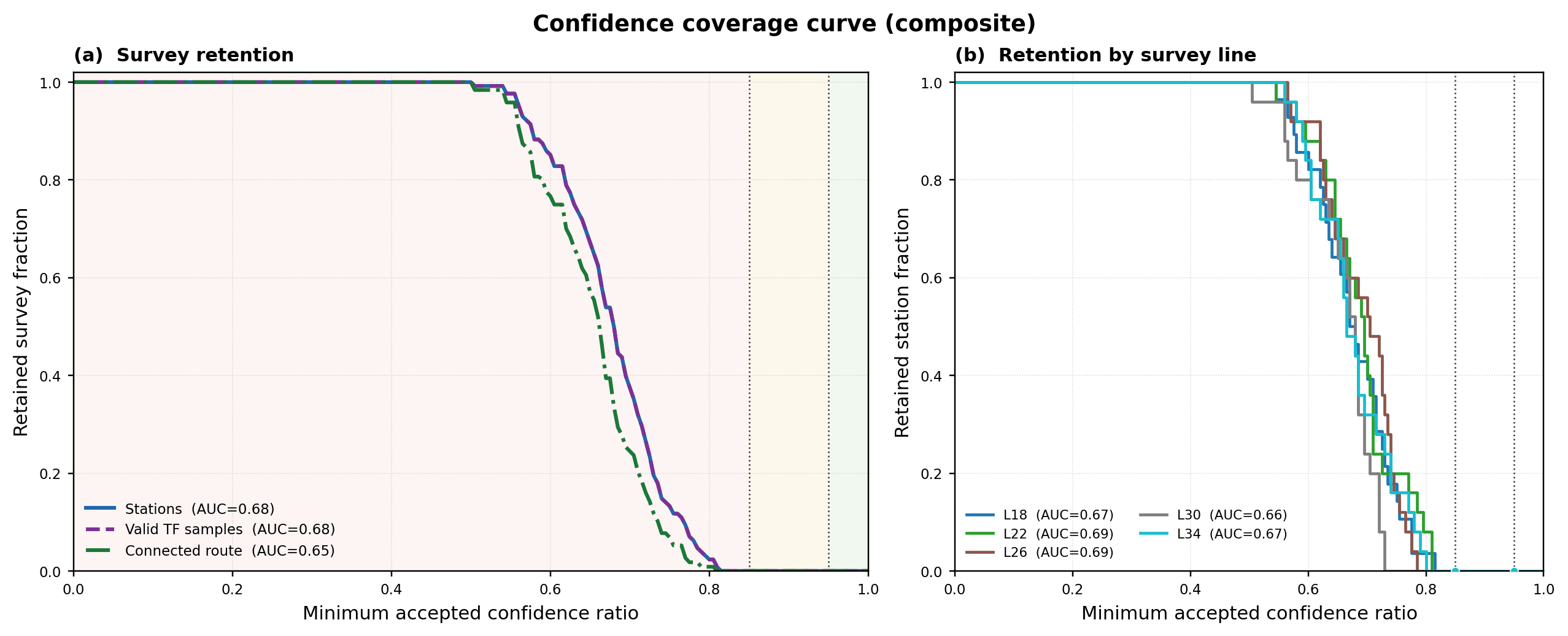
Retained station, valid-data, and connected-route fractions versus CR.#
Station and valid-data AUC are about 0.68, while connected-route AUC is about 0.65. The earlier loss of route coverage means isolated weak stations fragment otherwise retained line segments. All curves reach zero before 0.85, consistent with the risk and ranking views.
11.2.12. Station Confidence Profile#
plot_confidence_profile plots station confidence along the line. It
uses green, pink, and red markers for safe, recoverable, and rejected
stations.
>>> import matplotlib.pyplot as plt
>>> from pycsamt.emtools import plot_confidence_profile
>>> fig, ax = plt.subplots(figsize=(9.5, 4.2))
>>> _ = plot_confidence_profile(
...     "data/AMT/WILLY_DATA/L18PLT",
...     method="composite",
...     ci_hi=0.95,
...     ci_lo=0.85,
...     shade_mode="score",
...     station_label_step=2,
...     show_errorbars=True,
...     ax=ax,
... )
>>> fig.tight_layout()
>>> fig.savefig("confidence_profile_l18plt.png", dpi=200)
>>> plt.close(fig)
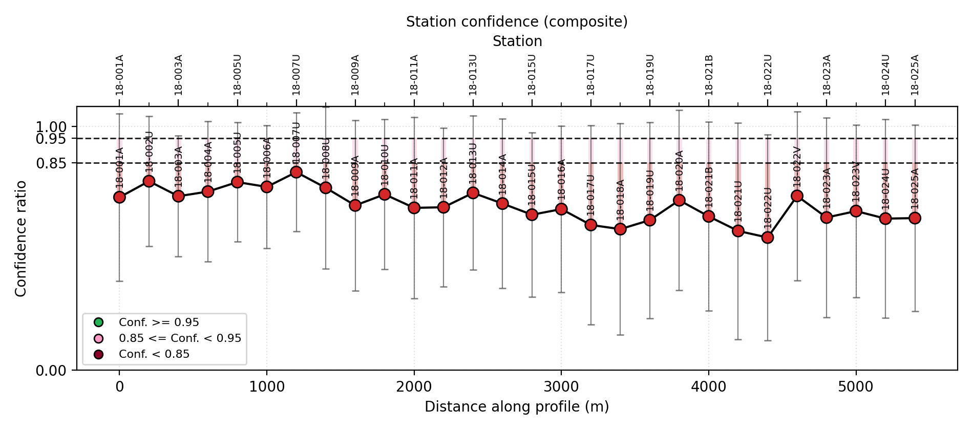
Every station is red because its composite score lies below the default
0.85 boundary; none is marginal and none is safe. The error bars are
component-score spread, as defined after
(1), not a confidence interval from repeat
measurements. L18 provides geographic coordinates, so pyCSAMT projects
their along-line separation into metres; the corrected route is about
2.4 km long, rather than the former 5 km display. spacing_m is used only
where coordinates are unavailable, or when force_spacing=True.
11.2.13. Frequency Confidence Pseudo-Section#
plot_frequency_confidence_psection shows confidence by station and
period. It can plot any metric column from the frequency table, not only
confidence.
>>> from pycsamt.emtools import plot_frequency_confidence_psection
>>> fig, ax = plt.subplots(figsize=(10.0, 4.8))
>>> _ = plot_frequency_confidence_psection(
...     "data/AMT/WILLY_DATA/L18PLT",
...     method="composite",
...     metric="confidence",
...     station_label_step=2,
...     ax=ax,
... )
>>> fig.savefig("frequency_confidence_psection.png", dpi=200)
>>> plt.close(fig)
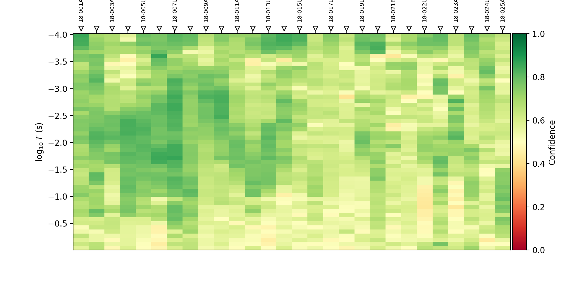
Change metric to "uncertainty", "offdiag", "diagonal",
"phase", or "spatial" to see which component is driving low
confidence at a given station and period, rather than only the combined
score.
11.2.14. Single-Station Spectrum#
plot_station_confidence_spectrum overlays the overall confidence
curve and component scores for one station.
>>> from pycsamt.emtools import plot_station_confidence_spectrum
>>> fig, ax = plt.subplots(figsize=(7.5, 4.2))
>>> _ = plot_station_confidence_spectrum(
...     "data/AMT/WILLY_DATA/L18PLT",
...     station="18-022U",
...     method="composite",
...     ax=ax,
... )
>>> fig.savefig("station_confidence_spectrum_18-022U.png", dpi=200)
>>> plt.close(fig)
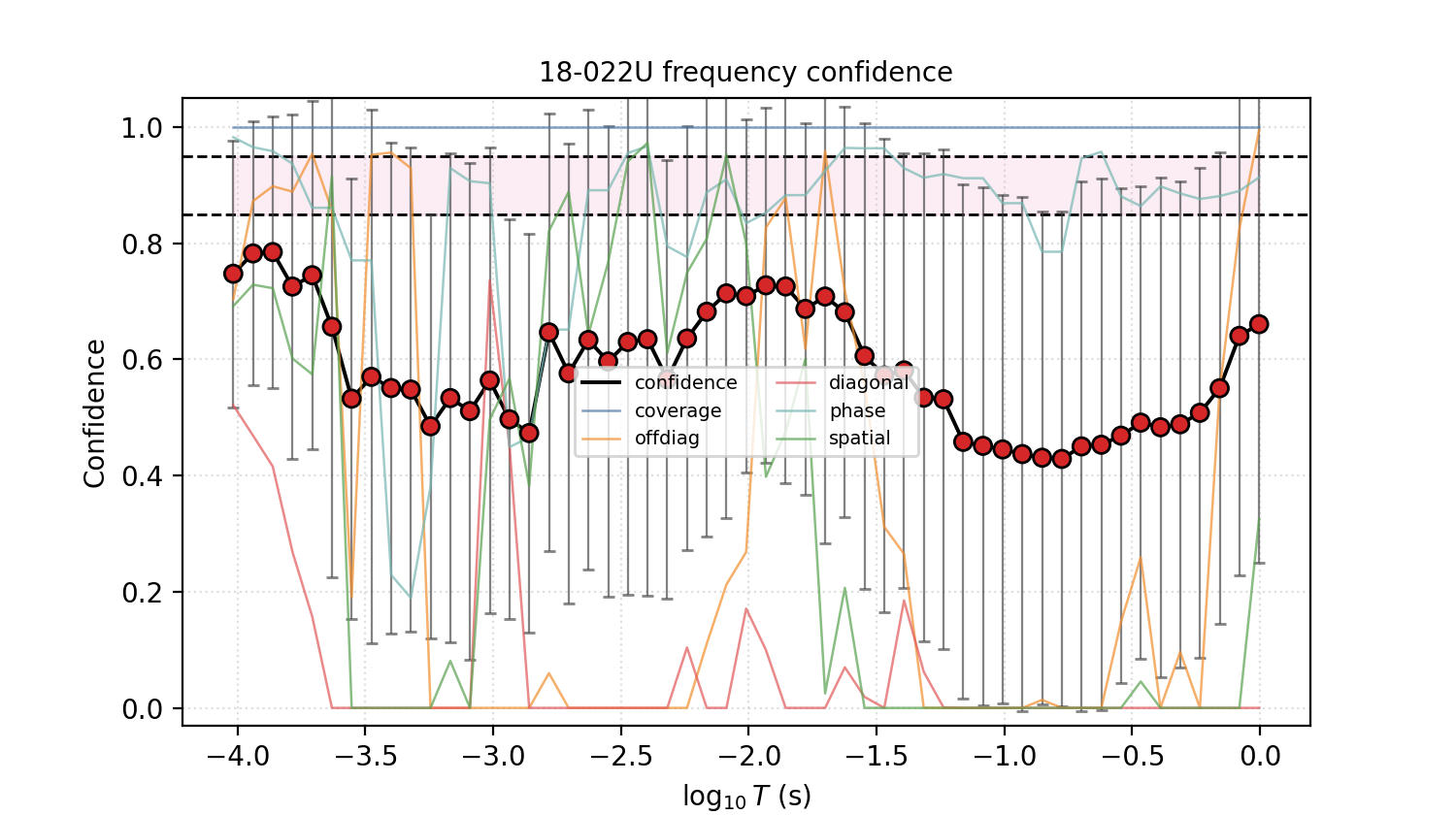
18-022U is this survey’s lowest-confidence station from the ranked
table above. Use this plot when you know a station is weak and want to
see whether the problem comes from uncertainty, diagonal leakage,
off-diagonal mismatch, phase jumps, or spatial incoherence, before
reaching for the dashboard’s split-panel view.
11.2.15. Single-Station Dashboard#
plot_station_confidence_dashboard breaks the same information into
separate panels. It is easier to read than the overlaid spectrum when
many score components overlap.
>>> from pycsamt.emtools import plot_station_confidence_dashboard
>>> fig = plot_station_confidence_dashboard(
...     "data/AMT/WILLY_DATA/L18PLT",
...     station="18-022U",
...     method="composite",
...     ci_hi=0.95,
...     ci_lo=0.85,
...     figsize=(11.0, 7.0),
... )
>>> fig.savefig("station_confidence_dashboard_18-022U.png", dpi=200)
>>> plt.close(fig)
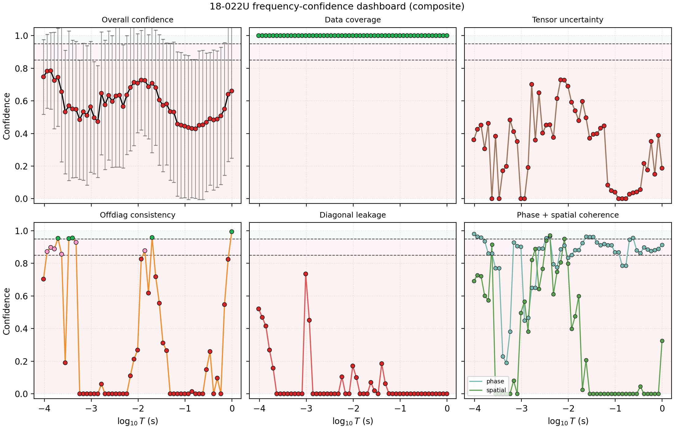
Split into six panels, the story reads clearly: “Data coverage” stays a flat, uninformative 1.0 throughout (top-middle), while “Offdiag consistency”, “Diagonal leakage”, and “Phase + spatial coherence” (bottom row) all repeatedly collapse toward zero – the composite penalty is concentrated in tensor-shape and spatial diagnostics, not missing data. Use dashboards for station-by-station review before deciding whether a low-confidence station should be edited, down-weighted, or retained.
11.2.16. Period-Band Summary#
plot_confidence_band_summary collapses the frequency table by
period. It plots median and mean confidence and shades the fraction of
stations in rejected or recoverable bands.
>>> from pycsamt.emtools import plot_confidence_band_summary
>>> fig, ax = plt.subplots(figsize=(8.5, 4.2))
>>> _ = plot_confidence_band_summary(
...     "data/AMT/WILLY_DATA/L18PLT",
...     method="composite",
...     ci_hi=0.95,
...     ci_lo=0.85,
...     ax=ax,
... )
>>> fig.savefig("confidence_band_summary.png", dpi=200)
>>> plt.close(fig)
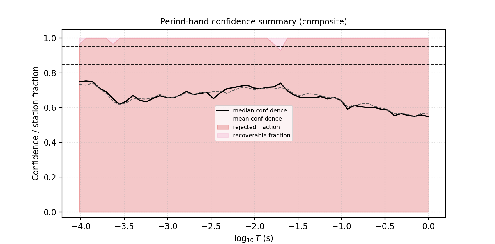
This view is useful when deciding whether a whole period band should be edited, down-weighted, or treated cautiously – it is also the figure that makes the “1479 of 1484 rejected cells” number from the frequency table above legible instead of abstract: the rejected-fraction shading runs high across nearly the entire period range shown here.
11.2.17. Coverage And SNR Quicklook#
plot_qc_quicklook combines three first-pass plots: a presence
pseudo-section, an SNR pseudo-section, and an SNR histogram.
>>> from pycsamt.emtools.qc import plot_qc_quicklook
>>> fig = plot_qc_quicklook(
...     "data/AMT/WILLY_DATA/L18PLT",
...     figsize=(10.0, 8.0),
... )
>>> fig.savefig("qc_quicklook_l18plt.png", dpi=200)
>>> plt.close(fig)
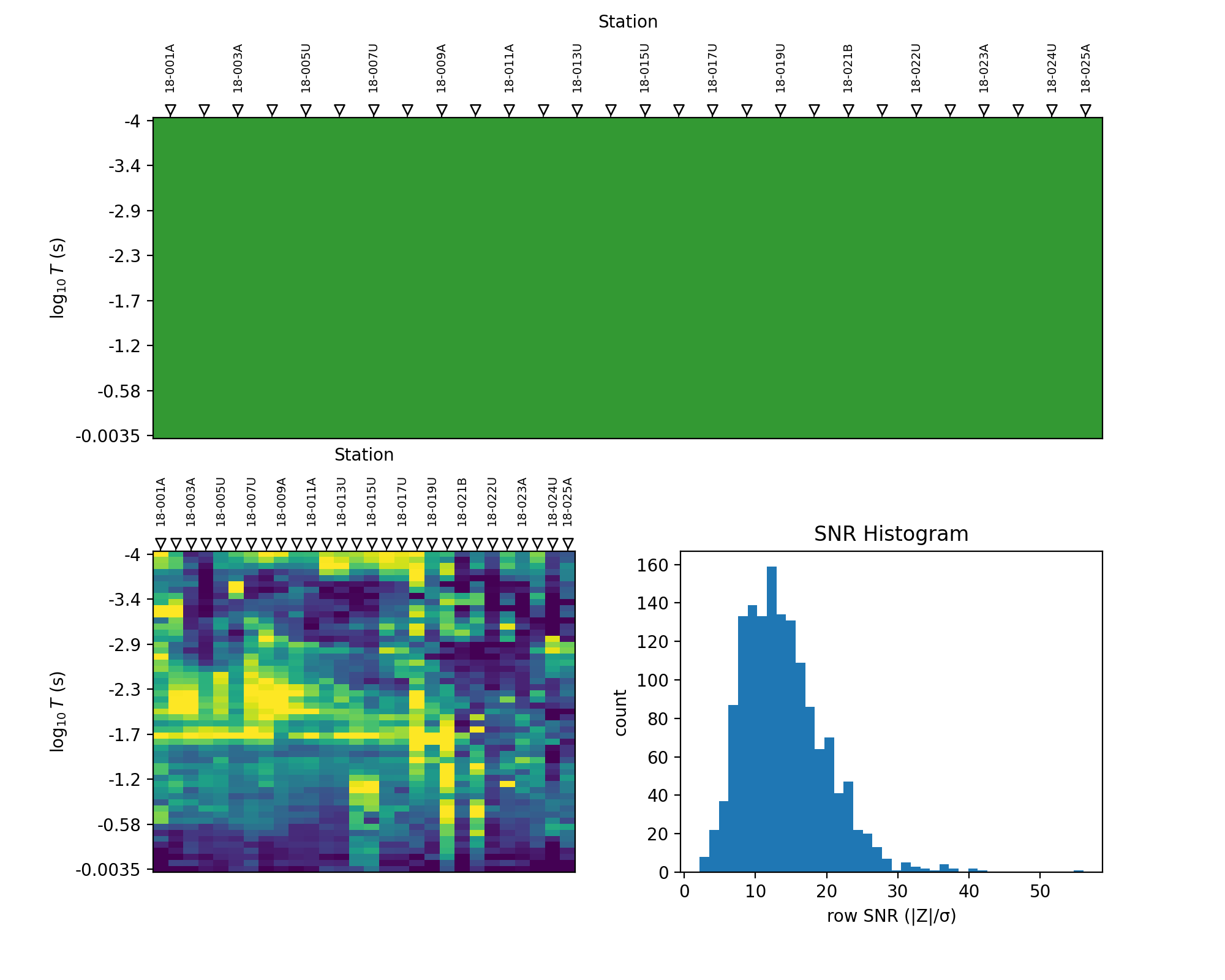
The top panel is solid green: 100% row presence everywhere, the same
frac_ok=1.0 finding from the station table. The bottom-left SNR
pseudo-section is where the real texture is – brighter (higher row
SNR, \(|Z|/\sigma\)) around the shorter periods and near a
few stations, fading elsewhere – and the histogram on the right shows
the underlying distribution peaking in the low tens with a long tail. If
the SNR histogram says error tensors are not available, the survey can
still be inspected, but uncertainty-based scores will be missing from
the composite confidence ratio.
11.2.18. Coverage Pseudo-Section And SNR Histogram#
For more control, call the helper plots separately.
>>> from pycsamt.emtools.qc import plot_coverage_psection, plot_snr_hist
>>> fig, axes = plt.subplots(1, 2, figsize=(12.0, 4.5))
>>> _ = plot_coverage_psection(
...     "data/AMT/WILLY_DATA/L18PLT",
...     metric="presence",
...     ax=axes[0],
... )
>>> _ = axes[0].set_title("Finite-row presence")
>>> _ = plot_snr_hist(
...     "data/AMT/WILLY_DATA/L18PLT",
...     bins=40,
...     ax=axes[1],
... )
>>> _ = axes[1].set_title("Row SNR distribution")
>>> fig.tight_layout()
>>> fig.savefig("coverage_and_snr.png", dpi=200)
>>> plt.close(fig)
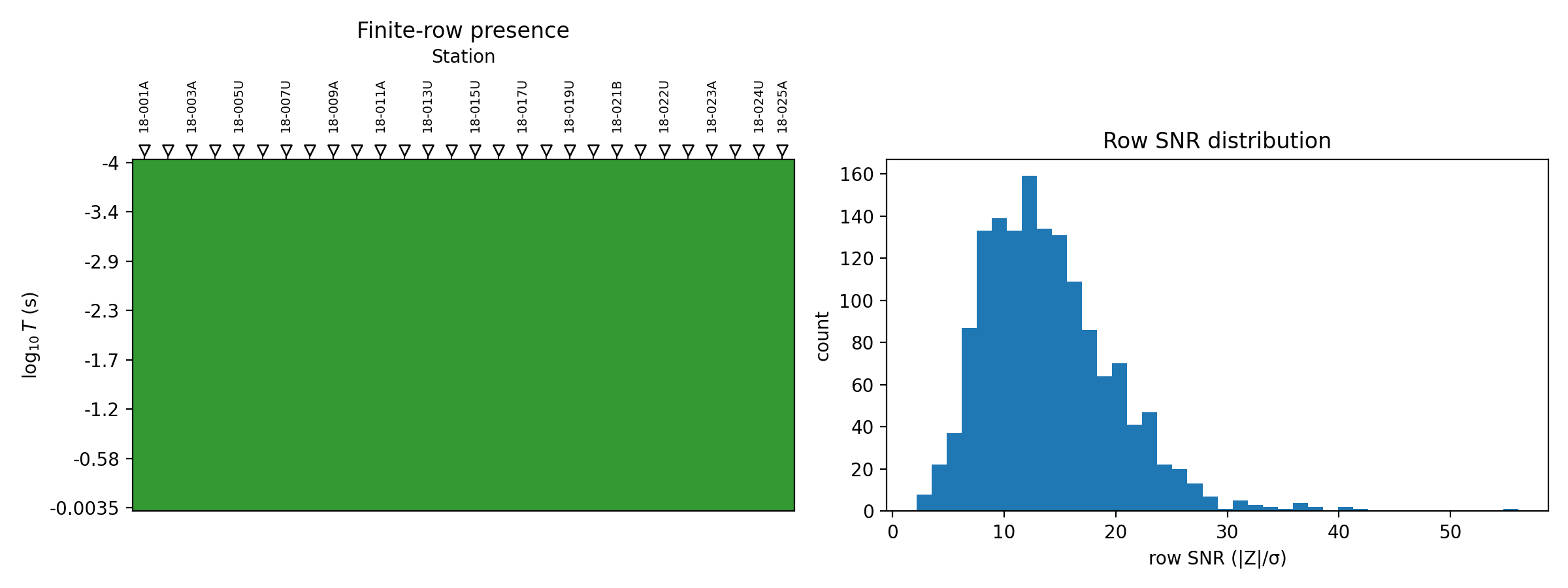
metric="presence" shows finite rows. metric="snr" colours by
row SNR when z_err exists. metric="offdiag" shows an
off-diagonal amplitude proxy.
11.2.19. Consistency Fan#
Apparent resistivity is a nonlinear function of impedance, so a
symmetric error on \(Z\) does not become a symmetric error on
\(\rho_a\) – the uncertainty score above summarizes that error
as one number, but it cannot show its shape. plot_consistency_fan
shows the shape directly by Monte Carlo sampling: it draws
\(n_{\mathrm{draws}}\) complex Gaussian perturbations with standard
deviation equal to the reported error,
recomputes \(\rho_a^{(d)} = 0.2\,|Z^{(d)}|^2 / f\) for each draw, and
plots the requested percentiles of the resulting distribution – the
10/50/90 default draws a band around the median rather than
a single curve. It can compare xy and yx
apparent resistivity bands for one station, which is exactly
where the offdiag score above would flag a problem, but here you
see the two bands and can judge for yourself whether they merely
disagree or actually fail to overlap.
>>> import numpy as np
>>> from pycsamt.emtools.qc import overlay_noise_cone, plot_consistency_fan
>>> fig, ax = plt.subplots(figsize=(8.8, 4.5))
>>> _ = plot_consistency_fan(
...     "data/AMT/WILLY_DATA/L18PLT",
...     station="18-016A",
...     comps=("xy", "yx"),
...     pcts=(10.0, 50.0, 90.0),
...     n_draws=300,
...     ax=ax,
... )
>>> ax.set_yscale("log")
>>> period = np.logspace(-4, 0, 30)
>>> overlay_noise_cone(
...     ax,
...     period,
...     lo=np.full(period.size, 10.0),
...     hi=np.full(period.size, 100.0),
...     color="0.5",
...     alpha=0.20,
... )
>>> fig.savefig("consistency_fan_18-016A.png", dpi=200)
>>> plt.close(fig)
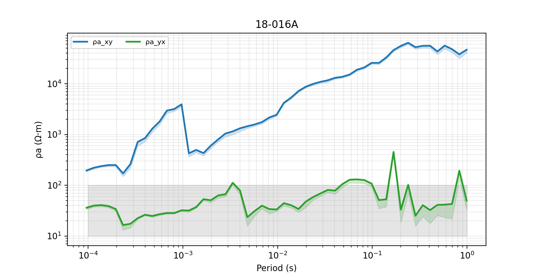
18-016A is the same station flagged elsewhere in this survey for
strong ratio anisotropy: on this log axis, \(\rho_{a,xy}\) climbs
into the tens of thousands of \(\Omega\,\mathrm{m}\) while
\(\rho_{a,yx}\) stays two to three decades lower throughout, and the
shaded Monte Carlo bands around each curve are genuinely propagated
from the EDI’s own error tensor rather than a linearized approximation.
The grey noise cone overlay is a visual reference band, not estimated
by the QC module – it happens to bracket most of this station’s real
\(\rho_{a,yx}\) values here while sitting far below
\(\rho_{a,xy}\). Supply project-specific lower and upper bounds when
you use it in a report.
11.2.20. XY/YX Crossover Map#
Away from a 1-D earth, rho_xy and rho_yx need not agree, but
which one is larger should not flip back and forth erratically with
period. plot_xyyx_crossover_map tracks the sign of
\(d(f) = \rho_{a,xy}(f) - \rho_{a,yx}(f)\) along each station’s
sounding and marks every period where it changes,
placing the marker at the log-period linearly interpolated between \(f_j\) and \(f_{j+1}\), weighted by how close each side came to zero. A station with one or two crossovers across a smooth sounding is unremarkable; a station peppered with them is a cheap, effective anisotropy and mode-consistency diagnostic worth following up with the consistency fan above.
>>> from pycsamt.emtools.qc import overlay_spectral_holes, plot_xyyx_crossover_map
>>> fig, ax = plt.subplots(figsize=(9.5, 4.8))
>>> _ = plot_xyyx_crossover_map(
...     "data/AMT/WILLY_DATA/L18PLT",
...     ax=ax,
... )
>>> overlay_spectral_holes(
...     ax,
...     "data/AMT/WILLY_DATA/L18PLT",
...     thresh_dec=0.30,
... )
>>> fig.savefig("xy_yx_crossover_map.png", dpi=200)
>>> plt.close(fig)
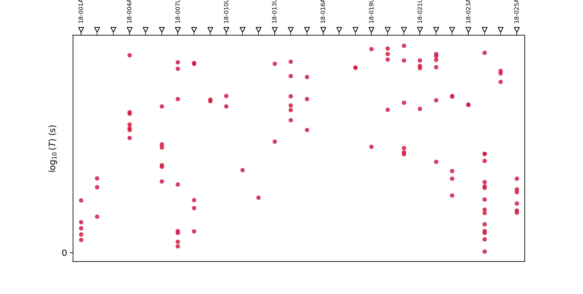
overlay_spectral_holes shades large gaps in log-period sampling on
top of a pseudo-section-style axis. L18PLT’s real frequency grid is
dense enough that the default 0.30-decade threshold finds nothing to
shade here – an honest negative result rather than a broken overlay.
Lower thresh_dec only when you intentionally want to reveal small
grid-spacing differences instead.
11.2.21. Propagation To Inversion#
For MARE2DEM exports created from EDI data, CR-derived uncertainty propagation can be enabled with:
>>> from pathlib import Path
>>> from pycsamt.models.mare2dem.edi import make_mt_data_from_edi
>>> out_path = Path("mare2dem_data_with_confidence.emdata")
>>> emd = make_mt_data_from_edi(
...     survey,
...     out_path,
...     confidence_weighting=True,
... )
>>> print(emd.n_mt_receivers, "receivers,", emd.n_mt_frequencies, "frequencies,", emd.n_data, "data")
28 receivers, 53 frequencies, 5936 data
The effective relative impedance error is inflated as confidence decreases:
The defaults are CR_min=0.05 and p=1. The usual propagation is
then:
Confidence weighting should increase uncertainty for low-confidence data. It should not make any datum artificially more precise.
11.2.22. Reading QC Results#
Use QC scores as evidence, not as an automatic delete button.
coverageis lowThe station or frequency is genuinely incomplete. Investigate loading, editing, or acquisition gaps.
uncertaintyis lowError tensors are large relative to impedance magnitude. This is a strong reason to down-weight or review.
offdiagis lowZxyandZyxamplitudes disagree beyond the selected tolerance. Compare with anisotropy, impedance, and tensor tools.diagonalis lowDiagonal leakage is high. Check dimensionality and coordinate orientation before calling it acquisition noise.
phaseis lowOff-diagonal phase changes abruptly with frequency. Check frequency editing and processing history.
spatialis lowThe station differs from neighbouring stations at the same frequency or in median response. Check station metadata and local geology.
11.2.23. Worked Example#
The gallery example applies the station, frequency, profile, dashboard, quicklook, fan, crossover, and hole-overlay workflows to the bundled L18PLT survey.
Open the rendered gallery page here: Quality-control confidence scoring (pycsamt.emtools.qc).