
11.17. Cross-Spectra Analysis#
pycsamt.emtools.spectra works below the processed impedance tensor.
Most emtools workflows start from an EDI Z tensor. This module
starts from the raw cross-power spectrum matrix stored in a
pycsamt.seg.spectra.Spectra object: one complex Hermitian
(n_channel, n_channel) matrix for each frequency in an EDI
>=SPECTRASECT block.
Use this module when you need to inspect spectra before they become impedance and tipper estimates:
channel power spectral density (PSD);
inter-channel squared coherence;
coherence-derived SNR;
frequency-band selection from coherence;
the full cross-power matrix at one frequency;
impedance and tipper recovered from spectra;
PSD and coherence pseudo-sections across multiple spectra stations.
Full function signatures and parameter defaults are maintained in the
API reference. The analysis and plotting
functions are exported through the public pycsamt.emtools namespace.
The Spectra container itself lives in pycsamt.seg.spectra.
11.17.1. When To Use This Page#
Use spectra tools only when your EDI file contains a
>=SPECTRASECT block. Many EDI files contain only final impedance and
tipper estimates. Those files are valid for most pyCSAMT workflows, but
they do not contain the raw cross-power matrices required here.
The bundled spectra examples are under data/MT/SPECTRA/:
data/MT/SPECTRA/spectra01.edi
data/MT/SPECTRA/spectra02.edi
They are de-identified field spectra files. Their identifying metadata was sanitized, while the numeric spectra blocks were kept for documentation and examples.
11.17.2. Workflow Map#
Task |
Use this |
Output |
|---|---|---|
Compute coherence cube |
|
Array with shape |
Build PSD table |
|
Tidy table with station, frequency, channel, and PSD. |
Build coherence table |
|
Tidy table with channel pairs and squared coherence. |
Estimate SNR from coherence |
|
Coherence table plus |
Restrict frequency band |
|
New |
Create coherence mask |
|
Boolean mask of frequencies that pass coherence criteria. |
Summarize spectra |
|
Per-frequency table with PSD and mean coherence. |
Plot single-station spectra |
|
PSD curves, pairwise coherence, and matrix image. |
Recover transfer functions |
|
Apparent resistivity/phase and induction tipper from spectra. |
Plot station sections |
|
Station-period pseudo-sections from multiple spectra objects. |
11.17.3. Loading Spectra#
Load spectra with Spectra.from_file. This is the one required
three-level import on this page because Spectra is a segmentation
container, not an emtools function.
>>> from pathlib import Path
>>> from pycsamt.seg.spectra import Spectra
>>> spectra_dir = Path("data/MT/SPECTRA")
>>> sp1 = Spectra.from_file(spectra_dir / "spectra01.edi")
>>> sp2 = Spectra.from_file(spectra_dir / "spectra02.edi")
>>> print(sp1.name, sp1.n_freq, sp1.n_chan)
SPECTRA01 51 7
>>> print(sp1.freq.min(), sp1.freq.max())
1.72 10400.0
>>> print(sp1.id_to_chtype)
{'31.003': 'HX', '32.003': 'HY', '33.003': 'HZ', '34.003': 'EX', '35.003': 'EY', '36.003': 'HX', '37.003': 'HY'}
A Spectra object exposes the core arrays used by this module:
>>> print(sp1.freq.shape)       # frequency vector
(51,)
>>> print(sp1.S.shape)          # cross-power matrix: (n_freq, n_chan, n_chan)
(51, 7, 7)
>>> print(sp1.bw.shape)         # bandwidth metadata
(51,)
>>> print(sp1.avgt.shape)       # averaging-time metadata
(51,)
>>> print(sp1.chan_ids)         # channel identifiers
['31.003', '32.003', '33.003', '34.003', '35.003', '36.003', '37.003']
The matrix sp1.S[k] is the full channel-by-channel
cross-power spectrum matrix at one frequency.
11.17.4. Coherence Matrix#
coherence_matrix computes squared coherence for every
channel pair:
The result is real-valued and bounded between 0 and 1.
>>> import numpy as np
>>> from pycsamt.emtools import coherence_matrix
>>> coh = coherence_matrix(sp1)
>>> print(coh.shape)
(51, 7, 7)
>>> print(np.nanmin(coh), np.nanmax(coh))
3.26311824218168e-06 1.0
>>> print(np.diagonal(coh, axis1=1, axis2=2)[0])
[1. 1. 1. 1. 1. 1. 1.]
The diagonal is 1 because each channel is perfectly coherent with itself. The off-diagonal values are the useful ones for judging whether two channels carry a stable relationship at a given frequency.
11.17.5. PSD Table#
psd_table extracts the power spectral density values from
the diagonal of the cross-power matrix as a tidy table. It accepts one
Spectra object, a list of spectra, or a dictionary of station names
to spectra.
>>> from pycsamt.emtools import psd_table
>>> psd = psd_table(sp1)
>>> print(psd.head())
     station     freq    period     channel           psd
0  SPECTRA01  10400.0  0.000096  HX(31.003)  1.561000e-09
1  SPECTRA01   8800.0  0.000114  HX(31.003)  2.342000e-09
2  SPECTRA01   7200.0  0.000139  HX(31.003)  4.808000e-09
3  SPECTRA01   6000.0  0.000167  HX(31.003)  3.892000e-09
4  SPECTRA01   5200.0  0.000192  HX(31.003)  2.224000e-09
>>> psd_norm = psd_table({"spectra01": sp1, "spectra02": sp2}, normalize=True)
>>> print(psd_norm.groupby(["station", "channel"])["psd"].max().head())
station    channel
spectra01  EX(34.003)    1.0
           EY(35.003)    1.0
           HX(31.003)    1.0
           HX(36.003)    1.0
           HY(32.003)    1.0
Name: psd, dtype: float64
Expected columns:
station, freq, period, channel, psd
Set normalize=True when you want to compare channel shapes rather
than absolute units. Electric and magnetic channels often have very
different physical units and raw PSD magnitudes.
11.17.6. Coherence Table#
coherence_table converts the coherence cube into a tidy
table. By default it includes all upper-triangle channel pairs. Pass
pairs to focus on physically meaningful pairs.
>>> from pycsamt.emtools import coherence_table
>>> # Example channel-index pairs used by the bundled spectra example:
>>> # EX-HY and EY-HX.
>>> mt_pairs = [(3, 1), (4, 0)]
>>> coherence = coherence_table(sp1, pairs=mt_pairs)
>>> print(coherence.head())
     station     freq    period  ...        ch_j                   pair coherence
0  SPECTRA01  10400.0  0.000096  ...  HY(32.003)  EX(34.003)-HY(32.003)  0.956060
1  SPECTRA01   8800.0  0.000114  ...  HY(32.003)  EX(34.003)-HY(32.003)  0.976360
2  SPECTRA01   7200.0  0.000139  ...  HY(32.003)  EX(34.003)-HY(32.003)  0.986516
3  SPECTRA01   6000.0  0.000167  ...  HY(32.003)  EX(34.003)-HY(32.003)  0.985696
4  SPECTRA01   5200.0  0.000192  ...  HY(32.003)  EX(34.003)-HY(32.003)  0.997629

[5 rows x 7 columns]
>>> print(coherence.groupby("pair")["coherence"].describe())
                       count      mean       std  ...       50%       75%       max
pair                                              ...
EX(34.003)-HY(32.003)   51.0  0.797033  0.270587  ...  0.900658  0.959647  0.998137
EY(35.003)-HX(31.003)   51.0  0.728161  0.244365  ...  0.798813  0.938283  0.996734

[2 rows x 8 columns]
Expected columns:
station, freq, period, ch_i, ch_j, pair, coherence
Use channel indices after checking sp.id_to_chtype. Spectra files can
carry duplicate reference channels or project-specific channel ordering.
11.17.7. Coherence-Derived SNR#
snr_table estimates SNR from squared coherence:
>>> from pycsamt.emtools import snr_table
>>> mt_pairs = [(3, 1), (4, 0)]
>>> snr = snr_table(sp1, pairs=mt_pairs)
>>> print(snr[["station", "freq", "pair", "coherence", "snr", "snr_db"]].head())
     station     freq                   pair  coherence         snr     snr_db
0  SPECTRA01  10400.0  EX(34.003)-HY(32.003)   0.956060   21.758405  13.376271
1  SPECTRA01   8800.0  EX(34.003)-HY(32.003)   0.976360   41.301034  16.159609
2  SPECTRA01   7200.0  EX(34.003)-HY(32.003)   0.986516   73.161532  18.642828
3  SPECTRA01   6000.0  EX(34.003)-HY(32.003)   0.985696   68.909149  18.382769
4  SPECTRA01   5200.0  EX(34.003)-HY(32.003)   0.997629  420.809415  26.240854
>>> print(snr.groupby("pair")["snr_db"].mean())
pair
EX(34.003)-HY(32.003)    9.044718
EY(35.003)-HX(31.003)    6.879817
Name: snr_db, dtype: float64
The two pairs are not equally clean: EX-HY averages 9.0 dB while
EY-HX averages only 6.9 dB. Each pair mixes one electric and one
orthogonal magnetic channel, so a two-decibel gap between them already
signals that one horizontal direction is noisier than the other at this
site, before any impedance rotation is applied. This is not the same
table as the impedance-error SNR used in remove_noise. In this
spectra workflow, SNR is derived from channel coherence before transfer
functions are estimated.
11.17.8. Band Selection#
band_select returns a new Spectra object restricted to a
frequency interval. It slices all spectra arrays and metadata together.
>>> from pycsamt.emtools import band_select
>>> high_band = band_select(sp1, f_min=100.0, f_max=10400.0)
>>> print(sp1.n_freq, high_band.n_freq)
51 27
>>> print(high_band.freq.min(), high_band.freq.max())
115.0 10400.0
Use band selection when a frequency range is known to be more reliable or when you need a common band across stations.
11.17.9. Coherence Masks#
mask_low_coherence returns a boolean mask over frequencies. It does
not modify the Spectra object. A True value means the frequency
passes the coherence criterion.
>>> from pycsamt.emtools import mask_low_coherence
>>> pass_any = mask_low_coherence(
...     sp1,
...     pairs=mt_pairs,
...     threshold=0.5,
...     require_all=False,
... )
>>> pass_all = mask_low_coherence(
...     sp1,
...     pairs=mt_pairs,
...     threshold=0.5,
...     require_all=True,
... )
>>> print(f"any pair passes: {pass_any.sum()} / {pass_any.size}")
any pair passes: 44 / 51
>>> print(f"all pairs pass: {pass_all.sum()} / {pass_all.size}")
all pairs pass: 42 / 51
>>> only_one_fails = pass_any & ~pass_all
>>> print(f"only one pair fails at: {sp1.freq[only_one_fails].round(1).tolist()}")
only one pair fails at: [49.0, 5.6]
Use require_all=True when every requested channel pair must be
coherent before a frequency is accepted. Use False for a looser
screen where at least one pair is enough. Here the gap between the two
counts is small (44 versus 42): only two frequencies – 49.0
and 5.6 Hz – pass on one pair but fail on the other, so this
station’s coherence problems are broadly shared between EX-HY and
EY-HX rather than isolated to one channel pair.
11.17.10. Spectra Summary#
spectra_summary produces one row per frequency. It combines
frequency metadata, channel PSD values, and mean off-diagonal coherence.
>>> from pycsamt.emtools import spectra_summary
>>> summary = spectra_summary(sp1)
>>> print(summary.head())
      freq    period      bw  ...  psd_HX(36.003)  psd_HY(37.003)  mean_coherence
0  10400.0  0.000096  2600.0  ...    1.561000e-09    5.204000e-09        0.399433
1   8800.0  0.000114  2904.0  ...    2.342000e-09    7.303000e-09        0.530258
2   7200.0  0.000139  1800.0  ...    4.808000e-09    1.702000e-08        0.666576
3   6000.0  0.000167  1980.0  ...    3.892000e-09    1.619000e-08        0.690481
4   5200.0  0.000192  1300.0  ...    2.224000e-09    9.476000e-09        0.695167

[5 rows x 13 columns]
>>> print(summary[["freq", "period", "mean_coherence"]].head())
      freq    period  mean_coherence
0  10400.0  0.000096        0.399433
1   8800.0  0.000114        0.530258
2   7200.0  0.000139        0.666576
3   6000.0  0.000167        0.690481
4   5200.0  0.000192        0.695167
>>> print(summary.loc[summary["mean_coherence"].idxmin(), ["freq", "mean_coherence"]])
freq              1.72000
mean_coherence    0.10174
Name: 50, dtype: float64
Use this table for quick reporting and for finding frequency ranges
where average coherence collapses. Here the worst row is the very
lowest frequency in the file, 1.72 Hz, where mean coherence drops to
0.10 – essentially uncorrelated. Keep that frequency in mind: it
resurfaces below as the point where the recovered impedance also carries
the largest relative uncertainty.
11.17.11. PSD Plot#
plot_psd draws the auto-spectrum for selected channels.
>>> import matplotlib.pyplot as plt
>>> from pycsamt.emtools import plot_psd
>>> fig, ax = plt.subplots(figsize=(9, 5))
>>> _ = plot_psd(
...     sp1,
...     channels=None,
...     log_psd=True,
...     title=f"{sp1.name} PSD",
...     ax=ax,
... )
>>> fig.tight_layout()
>>> fig.savefig("spectra_psd_spectra01.png", dpi=200)
>>> plt.close(fig)
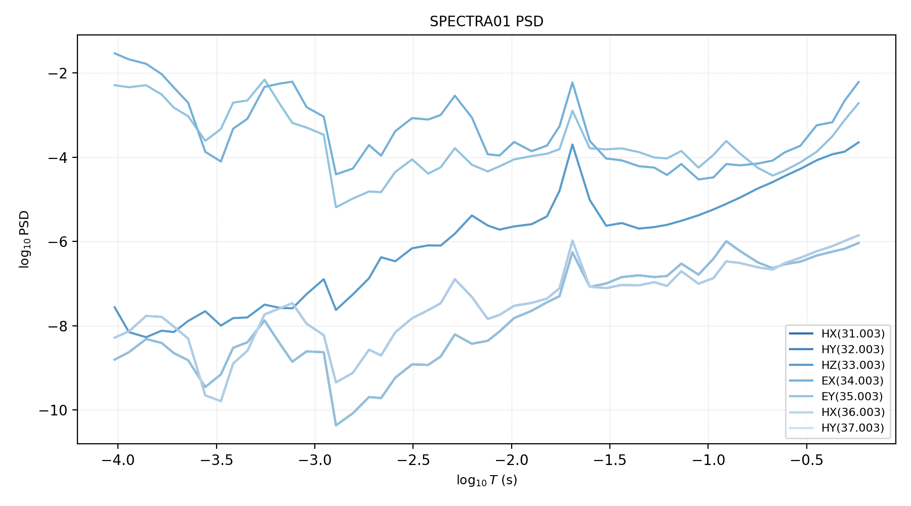
All seven channels share a sharp, narrow spike near
\(\log_{10}T \approx -1.7\) (about 0.02 s, 50 Hz) that stands
well above the smooth background trend on either side. A spike shared by
every channel at the same period, rather than a broad bump specific to
one sensor, is the signature of powerline harmonics rather than
natural-source signal – worth carrying into any later coherence or
frequency-band decision, since a bin dominated by mains noise can still
show artificially high coherence between channels that are both
contaminated the same way.
Pass a channel list when you want only a subset:
>>> ax = plot_psd(sp1, channels=[0, 1, 3, 4], log_psd=True)
>>> ax.figure.savefig("spectra_psd_subset_spectra01.png", dpi=200)
>>> plt.close(ax.figure)
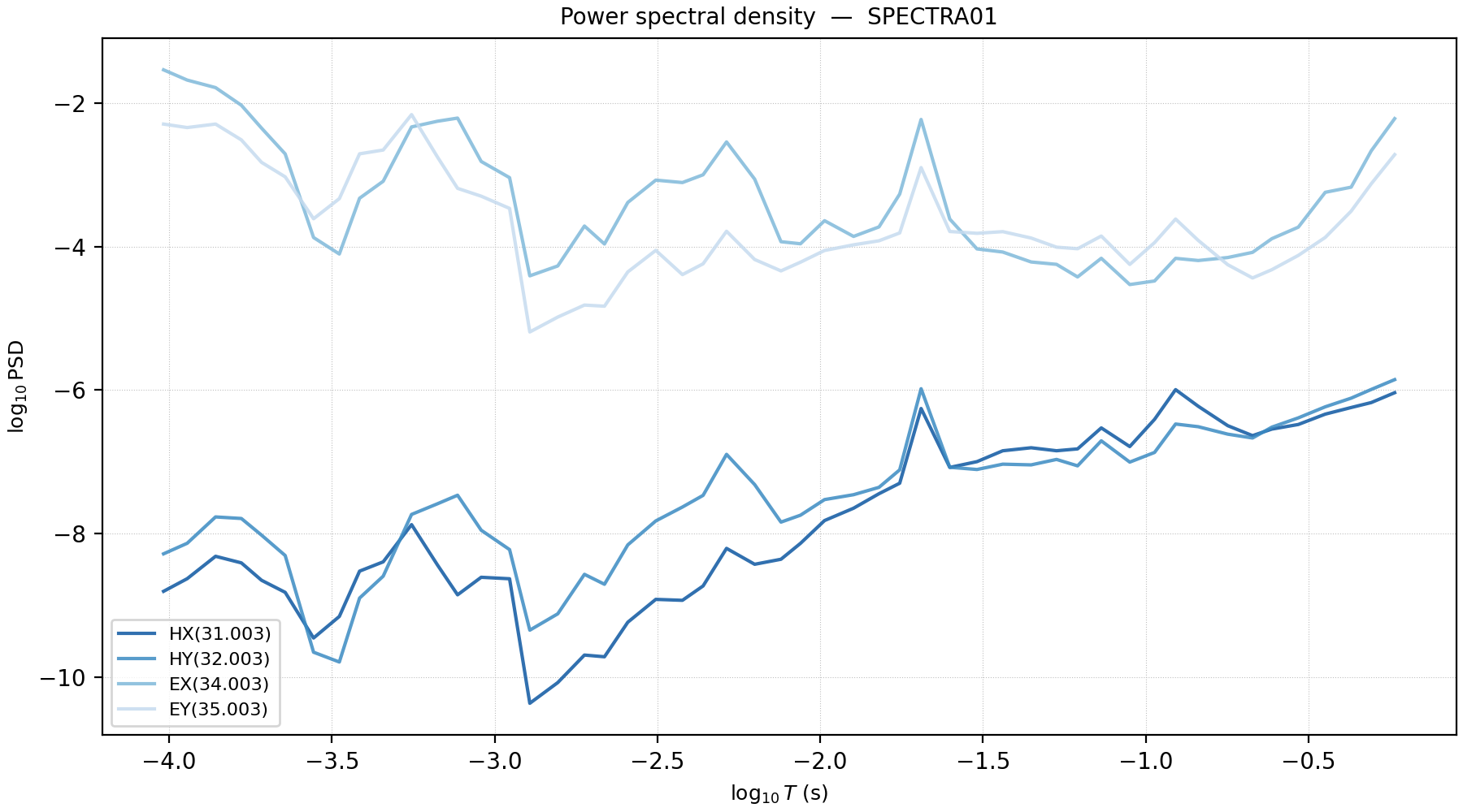
Channels 0 and 1 are HX(31.003) and HY(32.003); 3 and
4 are EX(34.003) and EY(35.003). Restricting to these four
makes the same 50 Hz spike easier to compare directly between the
magnetic pair (upper curves) and the electric pair (lower curves): it is
present in both, confirming it is a real, shared contaminant rather than
an artifact of one channel’s calibration. The x-axis follows the global
pyCSAMT plotting control, which is usually period-oriented for MT-style
figures.
11.17.12. Coherence Plot#
plot_coherence creates one axis per channel pair and draws the
threshold line.
>>> from pycsamt.emtools import plot_coherence
>>> axes = plot_coherence(
...     sp1,
...     pairs=mt_pairs,
...     threshold=0.5,
...     show_threshold=True,
...     title=f"{sp1.name} MT-pair coherence",
... )
>>> axes[0].figure.tight_layout()
>>> axes[0].figure.savefig("spectra_coherence_spectra01.png", dpi=200)
>>> plt.close(axes[0].figure)
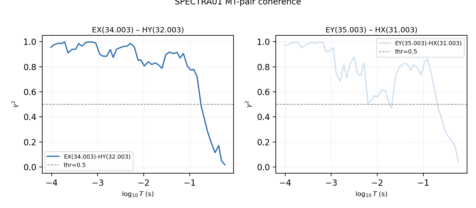
Use this plot before deciding on a band cut. A single mean coherence
number can hide whether failures are isolated, broad-band, or confined
to one channel pair. Both panels stay comfortably above the 0.5
threshold through most of the band and only drop below it toward the
right edge – long period, low frequency – confirming that the
0.10 mean coherence found above for 1.72 Hz is not an isolated
dip but the tail of a real, band-limited collapse. EY-HX (right
panel) also shows more mid-band scatter than EX-HY (left panel),
consistent with its lower average SNR reported earlier.
11.17.13. Full Spectral Matrix#
plot_spectra_matrix visualizes the complete cross-power
spectrum matrix at one frequency. The diagonal cells are auto-spectra.
Off-diagonal cells are cross-spectra.
>>> from pycsamt.emtools import plot_spectra_matrix
>>> fig = plot_spectra_matrix(
...     sp1,
...     freq_idx=0,
...     quantity="abs",
...     log_scale=True,
...     title="Cross-power matrix",
... )
>>> fig.savefig("spectra_cross_power_matrix.png", dpi=200, bbox_inches="tight")
>>> plt.close(fig)
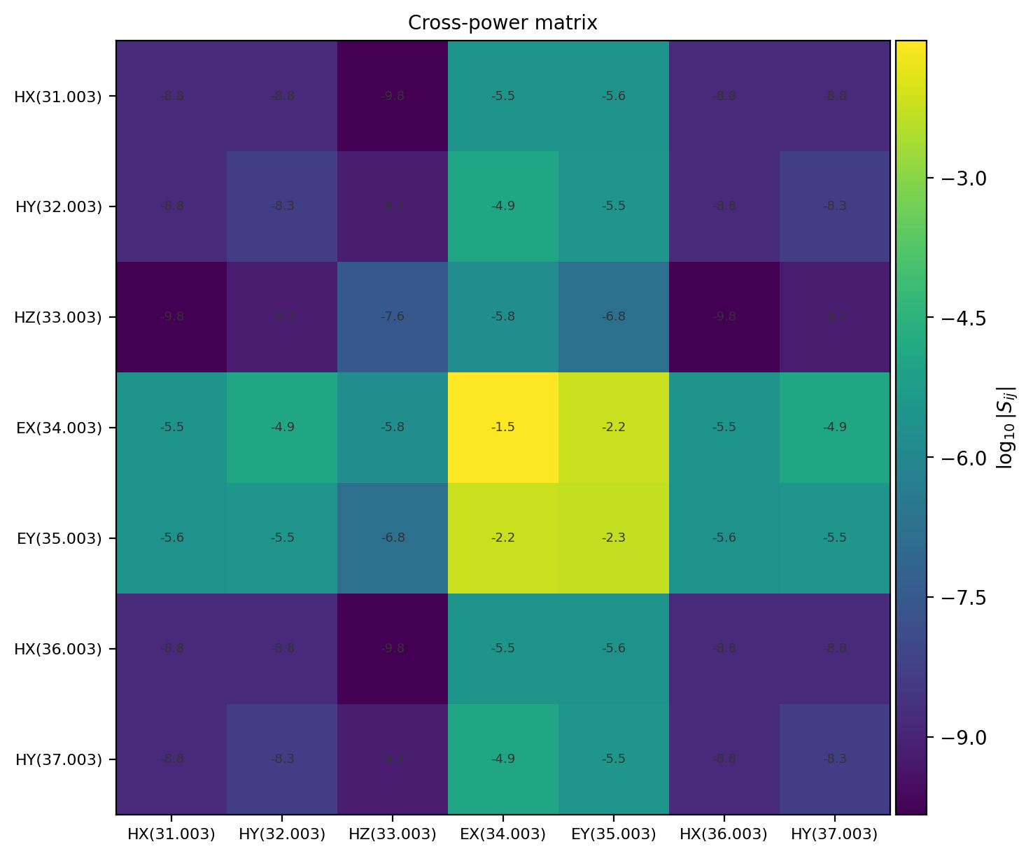
>>> diag = np.abs(np.diagonal(sp1.S[0]))
>>> offdiag = np.abs(sp1.S[0])[~np.eye(7, dtype=bool)]
>>> print("diagonal range:", diag.min(), diag.max())
diagonal range: 1.561e-09 0.02933
>>> print("off-diagonal range:", offdiag.min(), offdiag.max())
off-diagonal range: 1.4707397492418568e-10 0.0064268325791170255
At this frequency (index 0, the highest frequency in the file), the
electric diagonal cells (EX-EX, EY-EY) are the brightest
entries in the matrix – electric auto-power reaches 0.029, several
orders of magnitude above the 1.6e-9 magnetic auto-power floor,
matching the PSD plot above. The HX(31.003)/HX(36.003) row and
column are identical to within rounding, and likewise for
HY(32.003)/HY(37.003): this file genuinely carries two recordings
of the same two magnetic channels, useful to know before hard-coding a
channel index for e_labels or h_labels. HZ(33.003) has the
weakest cross-power with every other channel, including the electrics,
which is consistent with a 1-D/2-D setting where the vertical field
carries comparatively little energy at short period.
Available quantity values are "abs", "real", "imag", and
"phase". The log absolute view is usually the best first look because
electric and magnetic channel powers can span many orders of magnitude.
11.17.14. Recovering Impedance From Spectra#
Every table above works with coherence and power alone; recovering an
actual impedance tensor means going back to the full complex
cross-power matrix and solving for the linear system relating the
electric and magnetic fields. plot_z_from_spectra calls
Spectra.to_Z internally, which forms the per-frequency
least-squares solution directly from cross-power spectrum
sub-blocks:
where \(S_{HH}\) is the \(2\times2\) cross-power block between
the two horizontal magnetic channels and \(S_{EH}\) is the
\(2\times2\) cross-power block between the electric and magnetic
channels — this is the standard single-station cross-spectral
transfer-function estimator (Chave & Jones, 2012; Bendat & Piersol,
2011), the same estimator that ordinary EDI processing already applied
before writing the final Z block; this module just lets you redo
it yourself, or redo it differently, from the raw spectra. When
ridge is set, \(S_{HH}\) is stabilized by
ridge regularization before inversion,
which trades a small, deliberate bias for a solvable system when the
two magnetic channels are nearly collinear (for example, during strong
plane-wave-like source conditions) and \(S_{HH}\) is close to
singular. plot_z_from_spectra plots apparent resistivity and phase
from the resulting impedance.
>>> from pycsamt.emtools import plot_z_from_spectra
>>> fig = plot_z_from_spectra(
...     sp1,
...     e_labels=("EX", "EY"),
...     h_labels=("HX", "HY"),
...     ridge=None,
...     estimate_error=False,
...     show_error=True,
... )
>>> fig.savefig("spectra_impedance_spectra01.png", dpi=200, bbox_inches="tight")
>>> plt.close(fig)
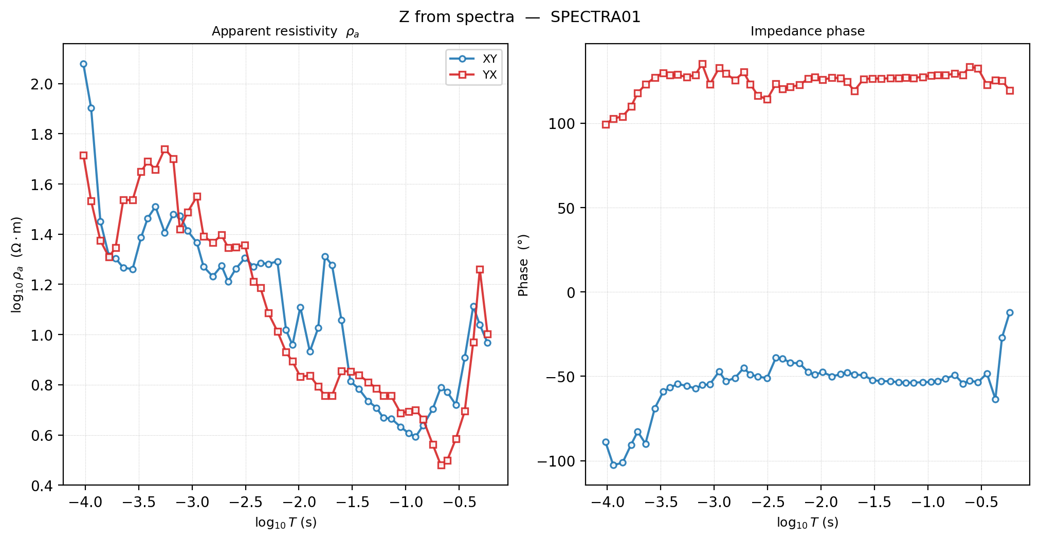
Both apparent-resistivity curves sit in a broadly similar 0.5-100
\(\Omega\cdot\mathrm{m}\) range and rise sharply again at the far
right of the plot – the longest periods, corresponding to the same
1.72 Hz region already flagged as the lowest-coherence part of the
band. XY phase runs negative (roughly -50 to -100 degrees)
while YX phase runs positive (roughly 100 to 135 degrees);
this quadrant offset between the two modes is the expected impedance
sign convention, not a data problem, but the two curves should still
track each other in shape if the site behaves close to 1-D or 2-D. For
programmatic access, call to_Z on the Spectra object:
>>> z_obj, tipper_obj = sp1.to_Z(
...     e_labels=("EX", "EY"),
...     h_labels=("HX", "HY"),
...     estimate_error=False,
... )
>>> print(z_obj.z.shape)
(51, 2, 2)
>>> print(z_obj.resistivity[:, 0, 1].min(), z_obj.resistivity[:, 0, 1].max())
3.9104053794314146 119.75913187624168
Use ridge when the magnetic cross-power block is poorly conditioned.
When estimate_error=True, per-component 1-sigma uncertainties come
from first-order error propagation under a complex-Wishart noise model,
where \(M\) is the effective degrees of freedom and \(E\) is the
residual electric power left unexplained by the magnetic fit. Errors
scale as \(1/\sqrt{M}\), so short, coarsely averaged records give
wide error bars even when the point estimate of \(Z\) looks clean.
\(M\) is resolved per frequency from whichever metadata the EDI
actually carries: an explicit segnum when it is nonzero, otherwise
round(avgt \times bw). A zero segnum is treated as “not
populated” rather than a literal zero count, because that is how most
real >=SPECTRASECT blocks leave the field – this file is typical:
>>> print("segnum unique:", np.unique(sp1.segnum))
segnum unique: [0]
>>> z_obj_err, tipper_obj_err = sp1.to_Z(
...     e_labels=("EX", "EY"),
...     h_labels=("HX", "HY"),
...     estimate_error=True,
... )
>>> print(z_obj_err.z_err is None)
False
>>> print(z_obj_err.z_err[:, 0, 1].min(), z_obj_err.z_err[:, 0, 1].max())
33.12781674552618 8363.127644544606
>>> rel_err = np.abs(z_obj_err.z_err[:, 0, 1]) / np.abs(z_obj_err.z[:, 0, 1])
>>> print(rel_err.min(), rel_err.max())
0.26120599954764967 556.645486781288
>>> worst = int(np.argmax(rel_err))
>>> print("worst freq:", sp1.freq[worst], "mean_coherence there:", summary["mean_coherence"].iloc[worst])
worst freq: 1.72 mean_coherence there: 0.1017396794696922
Every segnum entry in this file is 0, so every uncertainty here
comes from the avgt * bw fallback – and it still works, because
avgt and bw are genuinely populated. If segnum, avgt, and
bw were all missing, \(M\) could not be resolved at any
frequency and z_err would come back as None rather than an array
of NaN; keep estimate_error=False in that situation to skip the
computation outright. The relative error (\(|Z_{err}|/|Z|\)) peaks at
the same 1.72 Hz frequency already flagged twice above as the
lowest-coherence point in the survey – error propagation and the
independent coherence-based QC agree on exactly which frequency to
distrust, which is the kind of cross-check that makes either diagnostic
more convincing alone.
Treat a large avgt * bw product with some caution, though. It is an
upper bound on independent averages, not a guarantee that consecutive
windows are truly independent; real acquisition segments often overlap
or share correlated noise, so metadata-derived \(M\) can be
optimistic and error bars correspondingly too tight. Passing an explicit,
more conservative dof widens them accordingly:
>>> z_obj_dof, _ = sp1.to_Z(
...     e_labels=("EX", "EY"),
...     h_labels=("HX", "HY"),
...     estimate_error=True,
...     dof=np.full(sp1.n_freq, 24.0),
... )
>>> print(z_obj_dof.z_err[:, 0, 1].min(), z_obj_dof.z_err[:, 0, 1].max())
2610.623917771129 9164782.185755124
Forcing dof=24 at every frequency – a small, deliberately
conservative count – inflates the error bars by roughly two orders of
magnitude compared to the metadata-derived estimate above. Use this when
you have independent knowledge of the true averaging count (from
acquisition logs, for instance) and do not trust avgt * bw to reflect
genuinely independent samples.
11.17.15. Recovering Tipper From Spectra#
plot_tipper_from_spectra recovers induction tipper components from
the same spectra object when an HZ channel is available, using the
same magnetic sub-block already inverted for Z:
where \(S_{ZH}\) is the \(1\times2\) cross-power block between
the vertical and the two horizontal magnetic channels. Because
\(T\) reuses the same \(S_{HH}^{-1}\) as \(Z\), the same
ridge value stabilizes both simultaneously — there is no separate
tipper-specific regularization to tune.
>>> from pycsamt.emtools import plot_tipper_from_spectra
>>> axes = plot_tipper_from_spectra(
...     sp1,
...     h_labels=("HX", "HY"),
...     ridge=None,
...     estimate_error=False,
...     show_error=True,
... )
>>> axes[0].figure.savefig("spectra_tipper_spectra01.png", dpi=200, bbox_inches="tight")
>>> plt.close(axes[0].figure)
>>> print(tipper_obj.tipper.shape)
(51, 1, 2)
>>> print(np.abs(tipper_obj.tipper).min(), np.abs(tipper_obj.tipper).max())
0.0049976262815050534 2.523596990085329
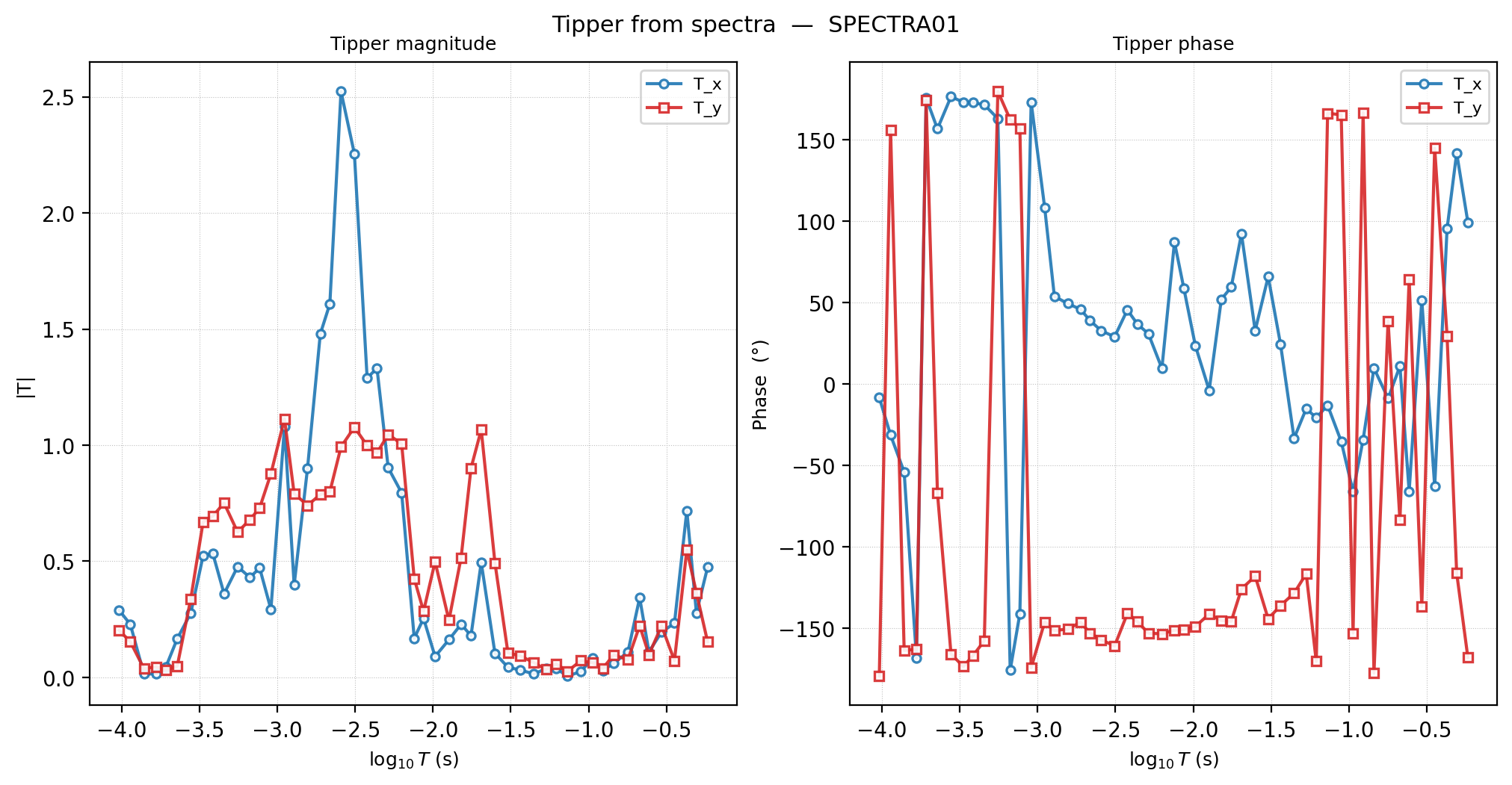
A physical induction-vector magnitude should stay below 1; the
2.52 maximum reported above, visible as the sharp spike around
\(\log_{10}T \approx -2.6\) with equally erratic phase on the right
panel, is a poorly conditioned single-frequency estimate rather than a
real deep-earth signal. This is exactly the situation ridge exists
for: pass a small positive value to stabilize \(S_{HH}\) before
inversion, or discard that frequency with band_select before trusting
the tipper curve. If no vertical magnetic channel is available, the
function returns axes with a no-tipper message rather than failing.
11.17.16. Multiple-Station Sections#
plot_psd_section and plot_coherence_section accept a list or
dictionary of Spectra objects. They build a common log-frequency grid
over the overlapping frequency range and interpolate each station onto
that grid.
>>> from pycsamt.emtools import plot_coherence_section, plot_psd_section
>>> spectra_sites = {
...     "spectra01": sp1,
...     "spectra02": sp2,
... }
>>> print("sp1 band:", sp1.freq.min(), sp1.freq.max())
sp1 band: 1.72 10400.0
>>> print("sp2 band:", sp2.freq.min(), sp2.freq.max())
sp2 band: 0.00042 320.0
>>> ax_psd = plot_psd_section(
...     spectra_sites,
...     channel=3,
...     log_psd=True,
...     title="EX PSD section",
... )
>>> ax_psd.figure.savefig("spectra_psd_section.png", dpi=200, bbox_inches="tight")
>>> plt.close(ax_psd.figure)
>>> ax_coh = plot_coherence_section(
...     spectra_sites,
...     pair=(3, 1),
...     threshold=0.5,
...     show_threshold=True,
...     title="EX-HY coherence section",
... )
>>> ax_coh.figure.savefig("spectra_coherence_section.png", dpi=200, bbox_inches="tight")
>>> plt.close(ax_coh.figure)
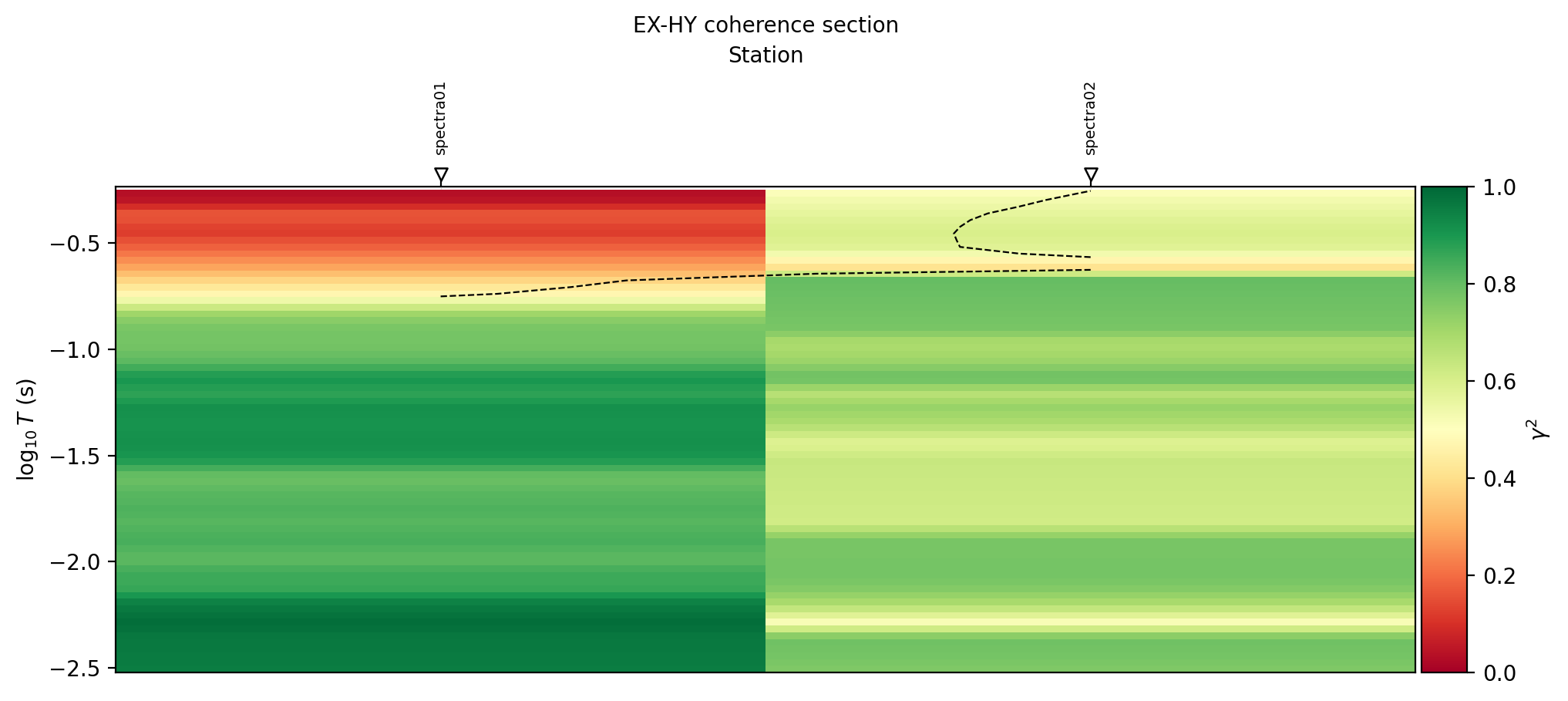
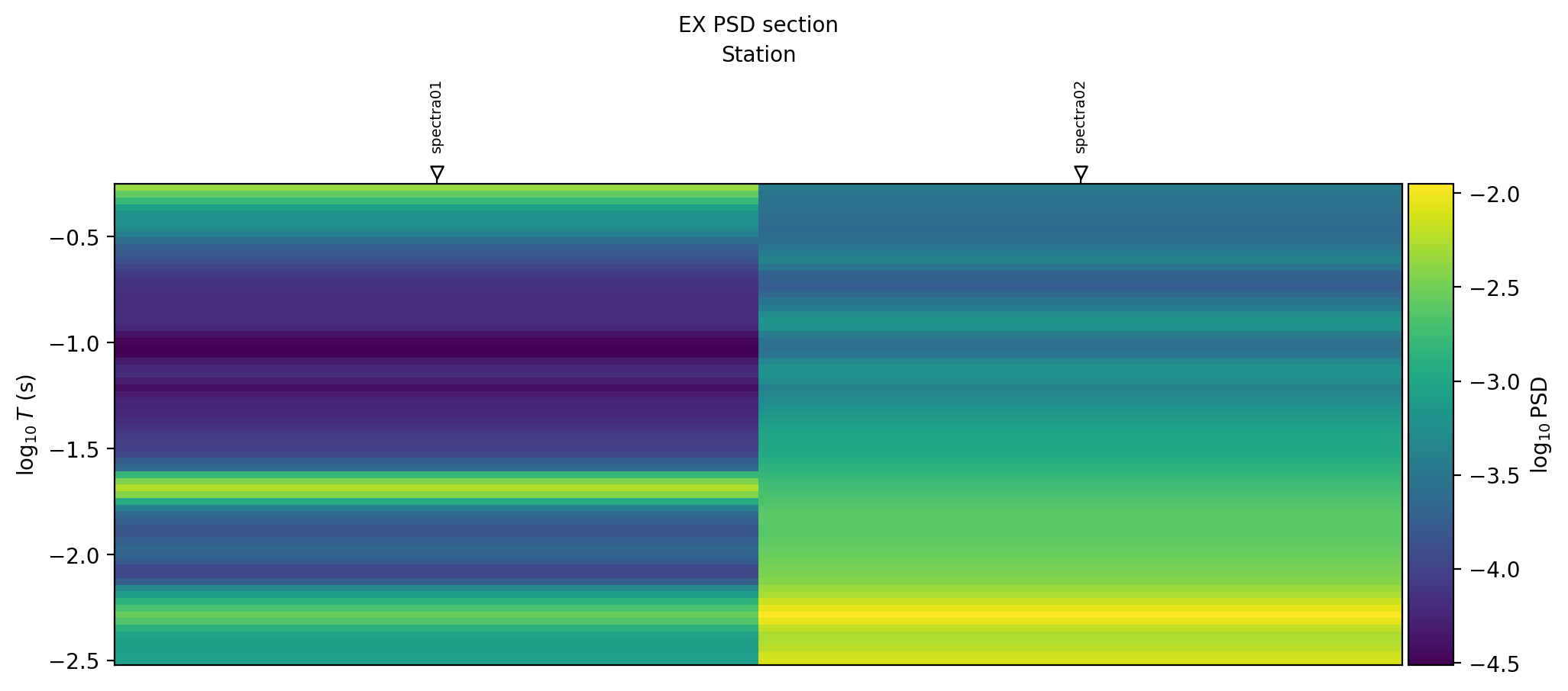
spectra01 and spectra02 are very different recordings – 1.72
to 10400 Hz versus a much longer-period 0.00042 to 320 Hz –
so the section functions use only the shared overlap, 1.72 to 320
Hz. They do not extrapolate outside a station’s spectra band, which is
why the PSD section’s 50 Hz powerline stripe is visible for both
stations (it falls inside the overlap) while each station otherwise keeps
its own PSD level. The coherence section makes the same long-period
collapse seen in the single-station coherence plot visible across
stations at once: spectra01 (left column) turns fully red – below
0.2 – at the longest periods in view, while spectra02 (right
column) only fades to a lighter yellow-green near the threshold over the
same interval. The degradation is real at both stations, just more
severe at spectra01, which is a stronger argument for a shared,
conservative band cut than either station’s plot alone.
11.17.17. Practical QC Recipe#
A compact spectra QC sequence is:
>>> full_mask = mask_low_coherence(
...     sp1,
...     pairs=mt_pairs,
...     threshold=0.5,
...     require_all=True,
... )
>>> print(f"full band pass: {full_mask.sum()} / {full_mask.size}")
full band pass: 42 / 51
>>> clean = band_select(sp1, f_min=100.0, f_max=10400.0)
>>> clean_mask = mask_low_coherence(
...     clean,
...     pairs=mt_pairs,
...     threshold=0.5,
...     require_all=True,
... )
>>> print(f"selected band pass: {clean_mask.sum()} / {clean_mask.size}")
selected band pass: 27 / 27
>>> coh = coherence_table(clean, pairs=mt_pairs)
>>> summary = spectra_summary(clean)
>>> print(coh.groupby("pair")["coherence"].describe())
                       count      mean       std  ...       50%       75%       max
pair                                              ...
EX(34.003)-HY(32.003)   27.0  0.947011  0.045600  ...  0.956582  0.986106  0.998137
EY(35.003)-HX(31.003)   27.0  0.858419  0.153881  ...  0.925313  0.988420  0.996734

[2 rows x 8 columns]
>>> print(summary[["freq", "mean_coherence"]].head())
      freq  mean_coherence
0  10400.0        0.399433
1   8800.0        0.530258
2   7200.0        0.666576
3   6000.0        0.690481
4   5200.0        0.695167
This sequence turns a visual coherence problem into a reproducible band
selection: define pairs, apply threshold, slice the spectra, and verify
the selected band. Restricting to 100-10400 Hz turns
require_all=True from a 42 / 51 pass rate into a clean 27 / 27
– every remaining frequency now clears both pairs – and lifts
EX-HY’s mean coherence from 0.80 (full band, from the earlier
table) to 0.95. That is the trade this recipe makes explicit: a
smaller, fully-passing band in exchange for dropping the low-frequency
tail this page has flagged repeatedly.
11.17.18. Pitfalls#
Do not use these functions on impedance-only EDIs. They require a
Spectra object with a real cross-power matrix.
Do not assume channel indices are universal. Always inspect
sp.id_to_chtype before hard-coding pairs such as (3, 1).
Do not confuse spectra coherence SNR with impedance-error SNR. The
spectra snr_table is derived from squared coherence. The
noise-removal SNR table is based on impedance errors.
Do not compare raw PSD values across electric and magnetic channels as if they shared units. Use log scaling or normalization when comparing shape.
Do not treat metadata-derived error bars as ground truth. A large
avgt * bw product can make uncertainties look tighter than the data
actually support; pass an explicit, conservative dof when you do not
trust the recording segments to be fully independent.
11.17.19. Worked Example#
The example loads the bundled de-identified spectra EDI files, plots PSD and coherence, builds PSD/coherence/SNR tables, selects a cleaner band, displays the full spectral matrix, recovers impedance and tipper from spectra, and builds multi-station PSD/coherence sections.
Open the rendered gallery page here: Cross-spectra analysis and visualization (pycsamt.emtools.spectra).