Cross-spectra analysis and visualization (pycsamt.emtools.spectra)

pycsamt.emtools.spectra works one level below the impedance tensor: instead of a processed Z (and, optionally, tipper), it operates directly on the raw cross-power spectral matrix stored in a Spectra object — one (n_chan, n_chan) complex Hermitian matrix per frequency, built from an EDI file’s >=SPECTRASECT block. That is a richer, less common EDI structure than the impedance-only files used elsewhere in this gallery (data/AMT/WILLY_DATA/, data/MT/kap03lmt_edis/), so this example uses two dedicated files bundled under data/MT/SPECTRA/ — de-identified copies of real field spectra (see data/MT/SPECTRA/README.md for the anonymization notes). It moves from a single channel’s power spectrum, through pairwise coherence and its tabular analysis siblings, a practical band-selection QC step, the full cross-power matrix at one frequency, apparent resistivity/phase and induction-tipper recovered directly from the spectra, and finishes with the two functions in this module that combine multiple stations into period-vs-station pseudo-sections.

1. Loading raw cross-spectra

Spectra.from_file() reads the >=SPECTRASECT block. spectra01 is a short-period/AMT-band file (51 frequencies, 10400–1.72 Hz); spectra02 is broadband/long-period (73 frequencies, 320–0.00042 Hz) — together they cover very different parts of the MT spectrum.

import numpy as np
from _datasets import dataset_path

from pycsamt.emtools import (
    band_select,
    coherence_table,
    mask_low_coherence,
    plot_coherence,
    plot_coherence_section,
    plot_psd,
    plot_psd_section,
    plot_spectra_matrix,
    plot_tipper_from_spectra,
    plot_z_from_spectra,
    psd_table,
    spectra_summary,
)

# snr_table is ambiguous at the top level (pycsamt.emtools.snr_table
# happens to resolve to this module's version today, but that depends
# on import order in emtools/__init__.py) -- import it explicitly.
from pycsamt.emtools.spectra import snr_table
from pycsamt.seg.spectra import Spectra

spectra_dir = dataset_path("mt_spectra")
sp1 = Spectra.from_file(spectra_dir / "spectra01.edi")
sp2 = Spectra.from_file(spectra_dir / "spectra02.edi")

print(
    f"{sp1.name}: {sp1.n_freq} freqs, {sp1.freq.min():.4g}"
    f"-{sp1.freq.max():.4g} Hz, {sp1.n_chan} channels"
)
print(
    f"{sp2.name}: {sp2.n_freq} freqs, {sp2.freq.min():.4g}"
    f"-{sp2.freq.max():.4g} Hz, {sp2.n_chan} channels"
)
print("channel types:", sp1.id_to_chtype)

SPECTRA01: 51 freqs, 1.72-1.04e+04 Hz, 7 channels
SPECTRA02: 73 freqs, 0.00042-320 Hz, 7 channels
channel types: {'31.003': 'HX', '32.003': 'HY', '33.003': 'HZ', '34.003': 'EX', '35.003': 'EY', '36.003': 'HX', '37.003': 'HY'}

Both files carry 7 channels: the usual EX/EY/HX/HY/ HZ plus a duplicated HX/HY pair — a local reference-field channel used for remote-reference-style noise rejection, not a second site.

2. Power spectral density — one station, one plot

plot_psd() draws the diagonal of the cross-power matrix (the auto-spectrum) per channel.

ax = plot_psd(sp1, title=f"{sp1.name} — power spectral density")

df_psd = psd_table(sp1)
for ch in df_psd["channel"].unique():
    sub = df_psd.loc[df_psd["channel"] == ch, "psd"]
    print(f"{ch:>12s}  psd range: {sub.min():.3e} - {sub.max():.3e}")

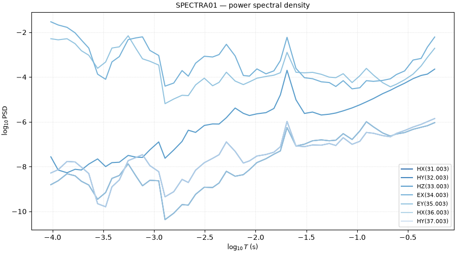
HX(31.003)  psd range: 4.282e-11 - 1.015e-06
HY(32.003)  psd range: 1.612e-10 - 1.400e-06
HZ(33.003)  psd range: 5.319e-09 - 2.257e-04
EX(34.003)  psd range: 2.967e-05 - 2.933e-02
EY(35.003)  psd range: 6.469e-06 - 6.968e-03
HX(36.003)  psd range: 4.282e-11 - 1.015e-06
HY(37.003)  psd range: 1.612e-10 - 1.400e-06

Reading this output. The E channels run roughly four orders of magnitude above the H channels in raw units (EX peaks near 0.029, HX near 1.0e-6) — an artefact of the different physical units (electric field vs. magnetic field), not a signal strength difference; the log-scaled y-axis in the plot is what makes the four channels comparable at all. The two HX traces (and the two HY traces) overlay each other exactly, confirming the duplicated reference channels really do carry the same physical signal.

3. Coherence between channel pairs

plot_coherence() grids every requested channel pair. The two pairs that matter for MT processing are the cross terms EX-HY and EY-HX.

mt_pairs = [(3, 1), (4, 0)]  # (EX, HY), (EY, HX) by channel index
axs = plot_coherence(
    sp1, pairs=mt_pairs, title=f"{sp1.name} — MT-relevant coherence"
)

df_coh = coherence_table(sp1, pairs=mt_pairs)
print(df_coh.groupby("pair")["coherence"].agg(["min", "max", "mean"]))

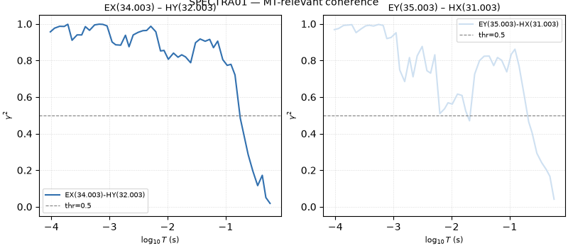
                            min       max      mean
pair
EX(34.003)-HY(32.003)  0.018285  0.998137  0.797033
EY(35.003)-HX(31.003)  0.041189  0.996734  0.728161

Reading this output. EX-HY coherence spans 0.018–0.998 (mean 0.80) and EY-HX spans 0.041–0.997 (mean 0.73) across the full 51-frequency band — some frequencies are excellent, others are essentially uncorrelated noise. That spread is exactly what section 5 below uses mask_low_coherence to quantify and act on.

4. Tabular analysis: SNR and the per-frequency summary

snr_table() converts coherence to a coherence-based SNR in dB; spectra_summary() gives one row per frequency with PSD for every channel plus the mean coherence across all channel pairs.

df_snr = snr_table(sp1, pairs=mt_pairs)
print(df_snr.groupby("pair")["snr_db"].mean())

df_sum = spectra_summary(sp1)
print(df_sum[["freq", "mean_coherence"]].head(3))
print(df_sum[["freq", "mean_coherence"]].tail(3))

pair
EX(34.003)-HY(32.003)    9.044718
EY(35.003)-HX(31.003)    6.879817
Name: snr_db, dtype: float64
      freq  mean_coherence
0  10400.0        0.399433
1   8800.0        0.530258
2   7200.0        0.666576
    freq  mean_coherence
48  2.34        0.136120
49  2.03        0.118128
50  1.72        0.101740

Reading this output. The mean coherence across all 21 channel pairs (not just the two MT-relevant ones) falls steadily from 0.40 at 10400 Hz down to 0.10 at 1.72 Hz — the low-frequency end of this short-period file is close to the edge of its useful range, which snr_table’s per-pair dB values make explicit (EX-HY: +9.0 dB mean SNR from the coherence-based estimator; the two duplicated-channel pairs HX-HX(RH) and HY-HY(RH) come back at the ceiling value, 120 dB, since they are the same signal measured twice).

5. Band selection and coherence masking

band_select() slices a Spectra to a frequency range; mask_low_coherence() flags frequencies that clear a coherence threshold.

mask_full_all = mask_low_coherence(
    sp1, pairs=mt_pairs, threshold=0.5, require_all=True
)
print(
    f"full band ({sp1.n_freq} freqs): "
    f"{mask_full_all.sum()}/{sp1.n_freq} pass thr=0.5 on both pairs"
)

sp1_hi = band_select(sp1, 100, 10400)
mask_hi_all = mask_low_coherence(
    sp1_hi, pairs=mt_pairs, threshold=0.5, require_all=True
)
print(
    f"restricted to [100, 10400] Hz ({sp1_hi.n_freq} freqs): "
    f"{mask_hi_all.sum()}/{sp1_hi.n_freq} pass"
)

full band (51 freqs): 42/51 pass thr=0.5 on both pairs
restricted to [100, 10400] Hz (27 freqs): 27/27 pass

Reading this output. Over the full band, 42 of 51 frequencies clear coherence 0.5 on both MT-relevant pairs simultaneously — the 9 that fail are exactly the lowest-frequency points, below 6.9 Hz. Restricting to [100, 10400] Hz with band_select keeps 27 frequencies, and every single one now passes: a practical two-line QC recipe (restrict, then verify) rather than a single opaque quality score.

6. The full cross-power matrix at one frequency

plot_spectra_matrix() colours the entire (n_chan, n_chan) complex matrix at a chosen frequency — every auto- and cross-spectrum at once.

fig = plot_spectra_matrix(sp1, freq_idx=0, quantity="abs")

M = sp1.S[0]
print(f"f = {sp1.freq[0]:.4g} Hz")
print(
    "log10|S_ij| range across the full 7x7 matrix:",
    f"{np.log10(np.abs(M[M != 0]).min()):.2f} to "
    f"{np.log10(np.abs(M).max()):.2f}",
)

f = 1.04e+04 Hz
log10|S_ij| range across the full 7x7 matrix: -9.83 to -1.53

Reading this output. At the top frequency (10400 Hz), log10|S_ij| spans roughly -9.8 (H-H cross terms) to -1.5 (the EX auto-power) — nearly ten orders of magnitude in one matrix, which is exactly why plot_spectra_matrix colours log10|S_ij| by default rather than the raw magnitude. The HX row/column and the duplicated HX(RH) row/column are numerically identical (likewise for HY/HY(RH)), the same structural duplication seen in section 2.

7. Apparent resistivity and phase, straight from spectra

plot_z_from_spectra() calls Spectra.to_Z() internally, recovering the impedance tensor by inverting the H-H cross-power block against the E-H cross-power block — the same computation a standard EDI’s Z tensor already encodes, but done here from the raw spectra.

fig = plot_z_from_spectra(sp1)

z1, _ = sp1.to_Z(estimate_error=False)
rho = z1.resistivity
print(
    f"rho_xy range: {np.nanmin(rho[:, 0, 1]):.2f}"
    f"-{np.nanmax(rho[:, 0, 1]):.2f} ohm.m"
)
print(
    f"rho_yx range: {np.nanmin(rho[:, 1, 0]):.2f}"
    f"-{np.nanmax(rho[:, 1, 0]):.2f} ohm.m"
)

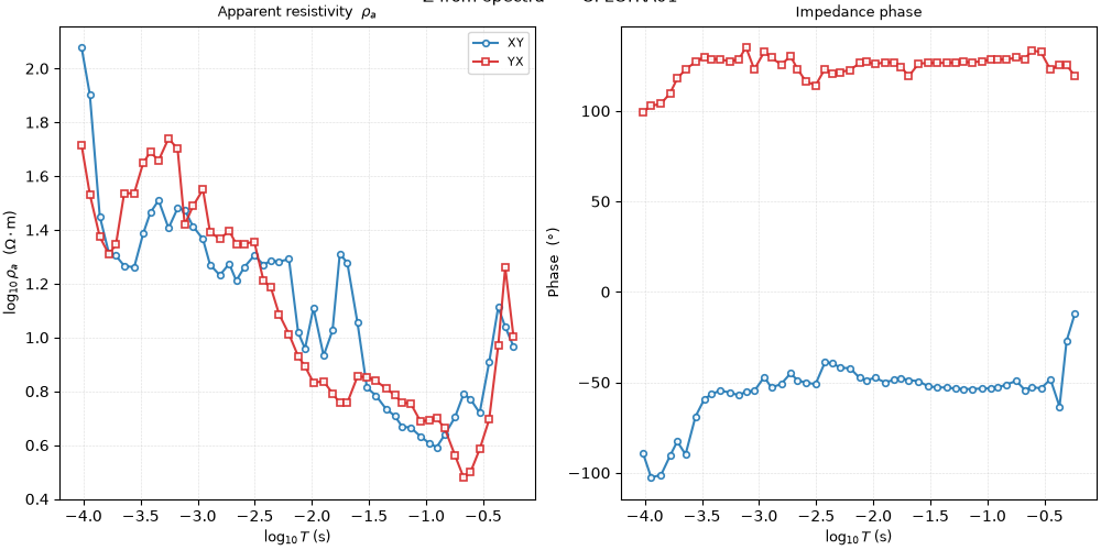
rho_xy range: 3.91-119.76 ohm.m
rho_yx range: 3.02-54.95 ohm.m

Reading this output. rho_xy runs 3.9–119.8 Ω·m and rho_yx runs 3.0–55.0 Ω·m over this station’s band — a factor of roughly 2-4 between the two apparent-resistivity curves at any given frequency, consistent with the 2-D/3-D structural complexity documented elsewhere in this gallery (see /emtools/ss), now confirmed from the spectra directly rather than from a pre-computed Z tensor.

8. Induction tipper, straight from spectra

plot_tipper_from_spectra() recovers T_x/T_y the same way, from the HZ cross-powers.

axs = plot_tipper_from_spectra(sp1)

_, tip1 = sp1.to_Z(estimate_error=False)
T = tip1.tipper[:, 0, :]
amp = np.abs(T)
print(f"|T_x| range: {amp[:, 0].min():.3f}-{amp[:, 0].max():.3f}")
print(f"|T_y| range: {amp[:, 1].min():.3f}-{amp[:, 1].max():.3f}")

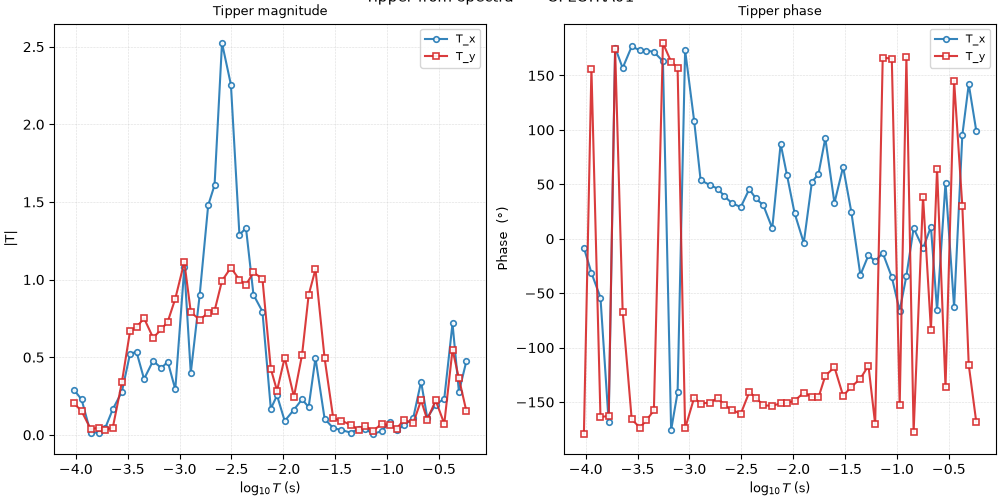
|T_x| range: 0.005-2.524
|T_y| range: 0.025-1.114

Reading this output. |T_x| reaches as high as 2.5 — a large tipper magnitude (values near or above 1 are unusual for simple 1-D layering) that reinforces the same 2-D/3-D reading as the apparent resistivity split above.

9. Combining stations: PSD and coherence pseudo-sections

plot_psd_section() and plot_coherence_section() are the two functions in this module built for multiple stations at once. Fed a dict of Spectra objects with different frequency bands, both interpolate onto a common log-frequency grid spanning the overlap between them before assembling the pseudo-section.

sites = {"spectra01": sp1, "spectra02": sp2}
ax = plot_psd_section(sites, channel=3)  # EX
ax2 = plot_coherence_section(sites, pair=(3, 1))  # EX-HY

f_lo = max(sp1.freq.min(), sp2.freq.min())
f_hi = min(sp1.freq.max(), sp2.freq.max())
print(f"common overlap band: {f_lo:.4g}-{f_hi:.4g} Hz")

• 
• 

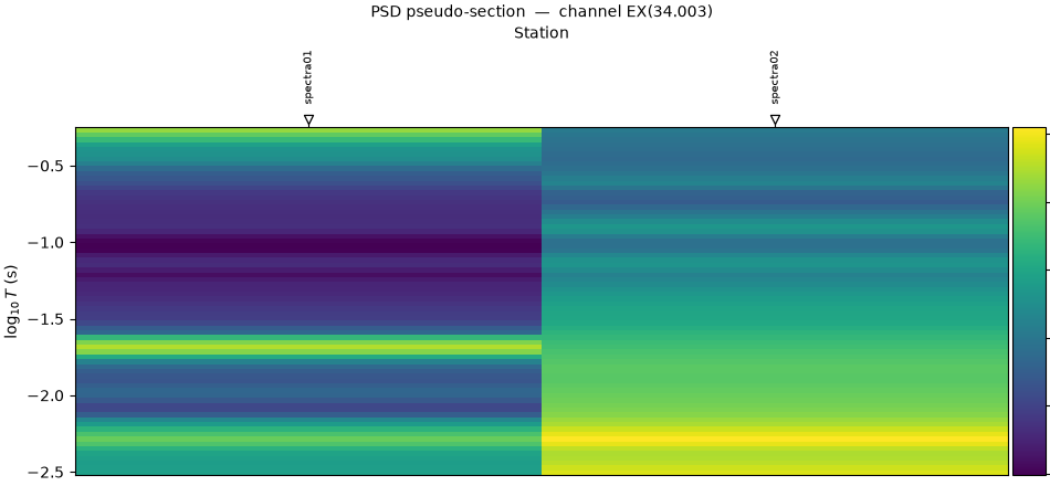
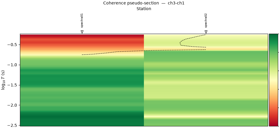
common overlap band: 1.72-320 Hz

Reading this output. spectra01 (10400–1.72 Hz) and spectra02 (320–0.00042 Hz) only overlap between 1.72 and 320 Hz — both pseudo-sections are built on that shared window, with each station’s own spectrum interpolated onto it, rather than silently padding the non-overlapping ends with extrapolated values.