Training a 1-D inverter end to end

The core idea of AI inversion: instead of iteratively fitting one sounding at a time, run the forward solver once over thousands of random earth models to build a (response → model) training set, then train a network to invert that mapping directly. Prediction on new data is then a single forward pass — milliseconds per sounding.

This first example walks the whole 1-D pipeline with EMInverter1D: generate the dataset, inspect its coverage, train a CNN, watch it converge, and validate the predicted layer models against the truth.

Build a synthetic training set

generate_dataset() samples random layered models and runs a forward solver on each. Here: 1200 four-layer MT soundings over a 24-frequency band, with 5% noise. The returned ForwardDataset holds the responses X (log10 apparent resistivity + phase at each frequency) and the target parameters y (log10 resistivity and thickness per layer).

# Use the predicted-vs-true model grid (4th figure) as the thumbnail.
import os

import numpy as np

from pycsamt.forward.batch import generate_dataset

# Train lighter while building the docs (PYCSAMT_DOCS_BUILD is set by the Sphinx
# build); full strength when the example is run directly.
_DOCS = bool(os.environ.get("PYCSAMT_DOCS_BUILD"))

FREQS = np.logspace(-1, 3, 24)
ds = generate_dataset(
    solver="mt1d",
    n_samples=256 if _DOCS else 1200,
    freqs=FREQS,
    n_layers=4,
    noise_level=0.05,
    seed=0,
    verbose=False,
)
print(ds)
print("X (responses):", ds.X.shape, " y (model params):", ds.y.shape)

train, val, test = ds.split()
print("train/val/test:", train.X.shape[0], val.X.shape[0], test.X.shape[0])

ForwardDataset(n=256, n_features=48, n_params=7, solver='mt1d')
X (responses): (256, 48)  y (model params): (256, 7)
train/val/test: 206 25 25

Coverage check: does the data span the target space?

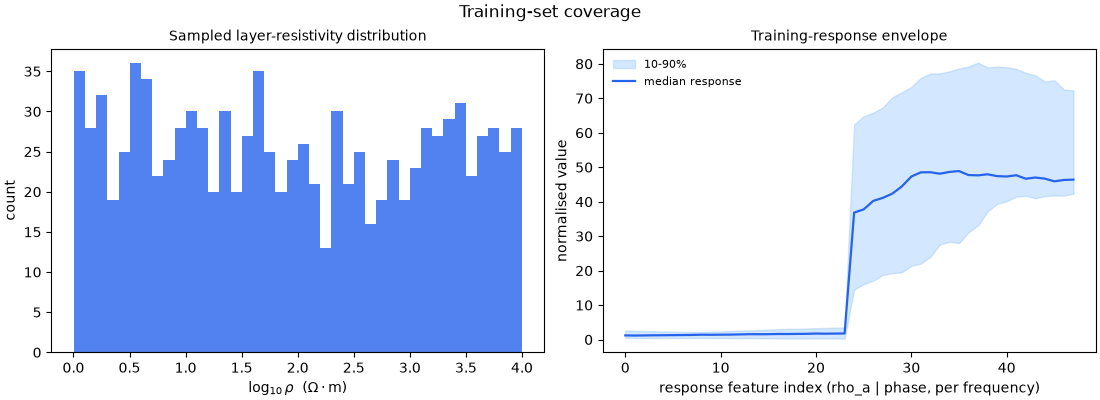
A network can only invert what it was trained on. Before training, plot the distribution of the sampled models and responses — real survey data must sit inside this envelope for predictions to be trustworthy.

import matplotlib.pyplot as plt

n_layers = 4
rho = ds.y[:, :n_layers]  # log10 resistivity per layer
fig, (axm, axr) = plt.subplots(
    1, 2, figsize=(11, 4.0), constrained_layout=True
)
axm.hist(rho.ravel(), bins=40, color="#2563eb", alpha=0.8)
axm.set_xlabel(r"$\log_{10}\rho$  ($\Omega\cdot$m)")
axm.set_ylabel("count")
axm.set_title("Sampled layer-resistivity distribution", fontsize=10)
p10, p50, p90 = np.percentile(ds.X, [10, 50, 90], axis=0)
feat = np.arange(ds.X.shape[1])
axr.fill_between(feat, p10, p90, color="#93c5fd", alpha=0.4, label="10-90%")
axr.plot(feat, p50, color="#2563eb", lw=1.6, label="median response")
axr.set_xlabel("response feature index (rho_a | phase, per frequency)")
axr.set_ylabel("normalised value")
axr.set_title("Training-response envelope", fontsize=10)
axr.legend(frameon=False, fontsize=8)
fig.suptitle("Training-set coverage", fontsize=12)

Text(0.5, 0.9895825, 'Training-set coverage')

Train the inverter

EMInverter1D wraps architecture, normalisation, and the training loop. We use a 1-D CNN; fit reports a history dictionary we plot next. (Epochs are kept low for a fast docs build — use more on real data.)

from pycsamt.ai.inversion.inv1d import EMInverter1D

inv = EMInverter1D(arch="cnn1d", n_layers=4, solver="mt1d")
inv.fit(train, epochs=6 if _DOCS else 25, batch_size=64, verbose=False)
print(
    "final train loss:",
    f"{inv._history['train_loss'][-1]:.4f}",
    " val loss:",
    f"{inv._history['val_loss'][-1]:.4f}",
)

final train loss: 0.6071  val loss: 0.9350

Convergence

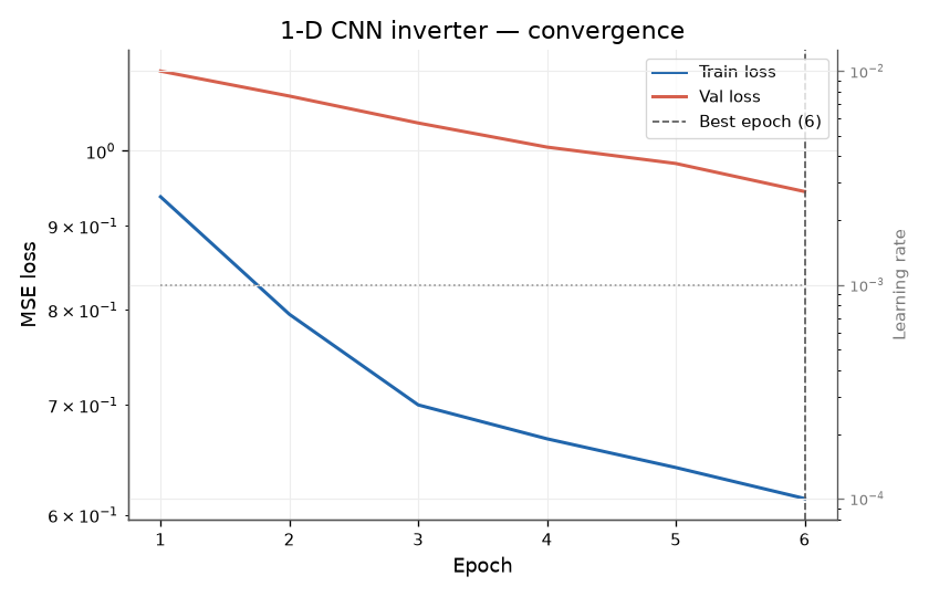
plot_convergence() shows train/validation loss (and the learning-rate schedule). A validation curve that tracks training and flattens smoothly — without diverging upward — indicates a healthy fit.

from pycsamt.ai.plot import plot_convergence

fig = plot_convergence(
    inv._history, smoothing=0.2, title="1-D CNN inverter — convergence"
)

Validate predicted models

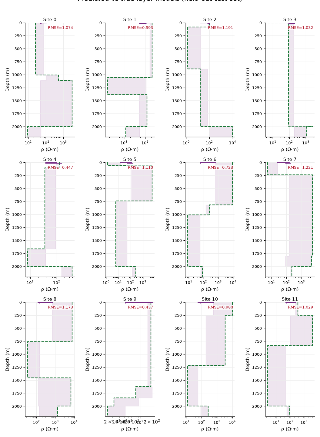
plot_compare() overlays predicted (dashed) and true (solid) resistivity-depth profiles for a grid of held-out test soundings, annotating each with its RMSE. This is the single most informative AI inversion figure — it shows where in the section the network is reliable.

from pycsamt.ai.plot import plot_compare, plot_profile_pair

y_pred = inv.predict(test.X)
fig = plot_compare(
    test.y[:12],
    y_pred[:12],
    n_cols=4,
    title="Predicted vs true layer models (held-out test set)",
)

A single sounding, larger

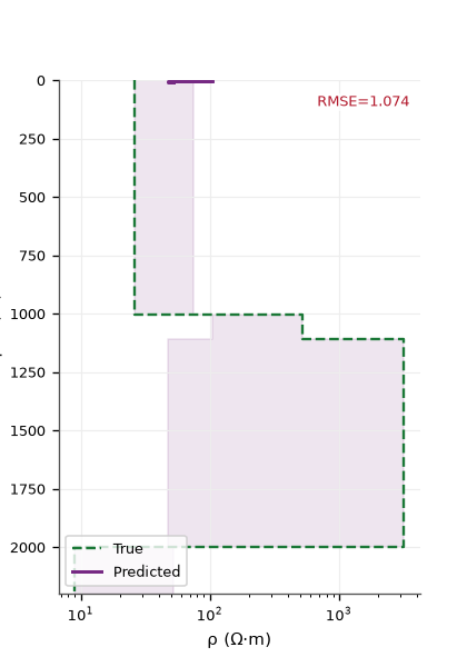
plot_profile_pair() is the one-station version — useful for a close look at a specific prediction.

ax = plot_profile_pair(test.y[0], y_pred[0])

Takeaway. With only 25 epochs on 960 training soundings the CNN already recovers the broad resistivity structure of unseen models. The next example turns this into a fair comparison across network architectures; Uncertainty and calibration then quantifies how much to trust each prediction.