
Note
Go to the end to download the full example code.
Step-by-step: from raw EDIs to sanitized EDIs#
This is the concrete, end-to-end version of the correction waves — a
teaching walkthrough of a real processing run. The key idea: every step is
a pure function that takes a Sites object and returns a new, cleaner
one. Chaining them takes the raw survey to a sanitized dataset, which we
finally write back out as EDIs — the artefact you would archive or invert.
We walk the WILLY_DATA L18PLT line through the whole chain, watching the data get cleaner at each stage, then apply the identical chain to L22PLT to show it generalises.
Start: load the raw line and look at its coverage#
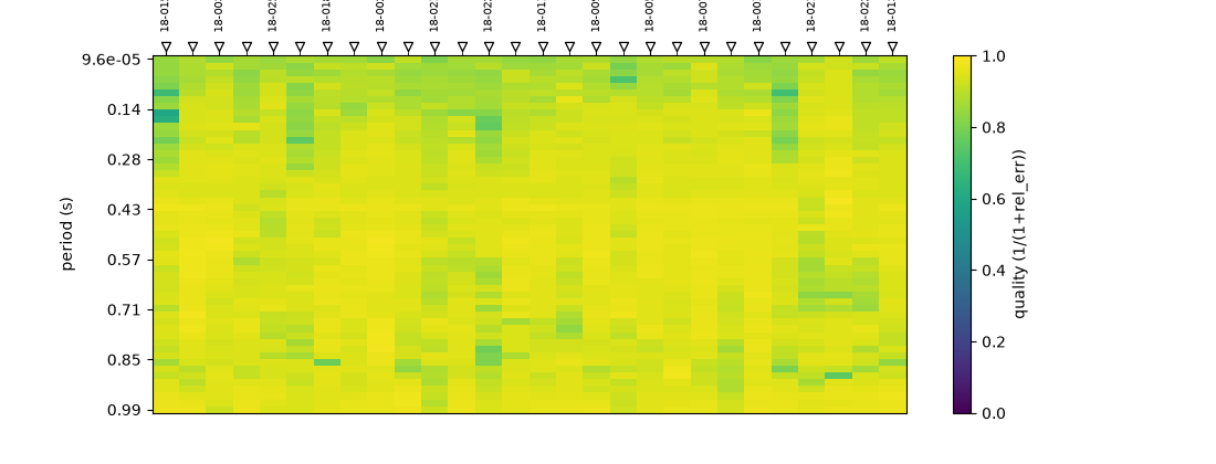
plot_coverage_quality_heatmap() maps data
quality over station x frequency — the “before” picture. Ragged edges and
low-quality (dark) cells are what the frequency-editing steps will trim.
import matplotlib.pyplot as plt
import numpy as np
from _corr_data import curves, demo_line, plot_before_after

from pycsamt.emtools import (
    correct_ss_ama,
    drop_duplicates,
    drop_low_confidence_frequencies,
    notch_powerline,
    plot_coverage_quality_heatmap,
    rotate_to_strike,
    select_band,
    smooth_logfreq,
)
from pycsamt.emtools._core import _iter_items
from pycsamt.site.export import write_sites


def n_freq(sites):
    """Frequencies retained per station — our sanitisation yardstick."""
    return np.array([len(np.asarray(ed.freq)) for ed in _iter_items(sites)])


raw = demo_line("L18PLT")
print(
    f"raw L18PLT: {len(n_freq(raw))} stations, "
    f"{n_freq(raw).min()}-{n_freq(raw).max()} frequencies each"
)
plot_coverage_quality_heatmap(raw, figsize=(11, 4.2))
raw L18PLT: 28 stations, 53-53 frequencies each

<Axes: xlabel='Station', ylabel='period (s)'>
Frequency editing — dropping the bad data#
The first three steps sanitise the frequency axis, each returning a new
Sites. drop_duplicates removes repeated frequencies; select_band
keeps the usable band (here 1 mHz - 1 kHz); and
drop_low_confidence_frequencies prunes the noisy bins whose composite
confidence falls below 0.5. Nothing is edited in place — each s is a
fresh, cleaner object.
s1 = drop_duplicates(raw, recursive=False)
s2 = select_band(s1, fmin=1e-3, fmax=1e3, recursive=False)
s3 = drop_low_confidence_frequencies(s2, threshold=0.5, recursive=False)

for label, s in [
    ("raw", raw),
    ("drop_duplicates", s1),
    ("select_band", s2),
    ("drop_low_confidence", s3),
]:
    nf = n_freq(s)
    print(f"  {label:<22} {nf.min():>3}-{nf.max():>3} frequencies/station")
raw                     53- 53 frequencies/station
drop_duplicates         53- 53 frequencies/station
select_band             39- 39 frequencies/station
drop_low_confidence     25- 39 frequencies/station
The sanitisation profile#
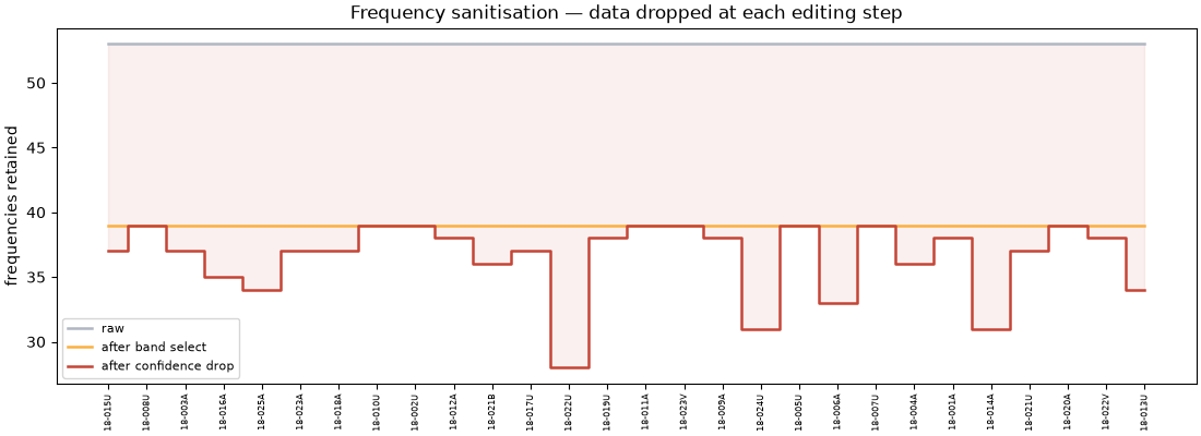
Plotting the retained frequency count per station at each stage makes the
trimming explicit: the flat drop at select_band (a fixed band for the
whole line) and the per-station drop at drop_low_confidence (each
station loses only its own bad bins).
stations = list(curves(raw))
x = np.arange(len(stations))
fig, ax = plt.subplots(figsize=(11, 4.0), constrained_layout=True)
ax.step(x, n_freq(raw), where="mid", lw=1.8, color="#b0b7c3", label="raw")
ax.step(
    x,
    n_freq(s2),
    where="mid",
    lw=1.8,
    color="#fbb040",
    label="after band select",
)
ax.step(
    x,
    n_freq(s3),
    where="mid",
    lw=1.8,
    color="#c44536",
    label="after confidence drop",
)
ax.fill_between(
    x, n_freq(s3), n_freq(raw), step="mid", color="#c44536", alpha=0.08
)
ax.set_xticks(x)
ax.set_xticklabels(stations, rotation=90, fontsize=6)
ax.set_ylabel("frequencies retained")
ax.set_title("Frequency sanitisation — data dropped at each editing step")
ax.legend(fontsize=8)
<matplotlib.legend.Legend object at 0x7f2dfbad2300>
Conditioning — cleaning what remains#
With the frequency axis trimmed, the next steps condition the surviving
data: notch the power line, smooth in log-frequency, remove static shift,
and rotate onto strike. Each, again, returns a new Sites.
s4 = notch_powerline(s3, recursive=False)
s5 = smooth_logfreq(s4, win=5, recursive=False)
s6 = correct_ss_ama(s5, recursive=False)
final = rotate_to_strike(s6, recursive=False)
print(
    "chain: raw -> drop_dup -> select_band -> drop_low_conf -> notch "
    "-> smooth -> static_shift -> rotate"
)
chain: raw -> drop_dup -> select_band -> drop_low_conf -> notch -> smooth -> static_shift -> rotate
Raw vs sanitised: apparent resistivity#
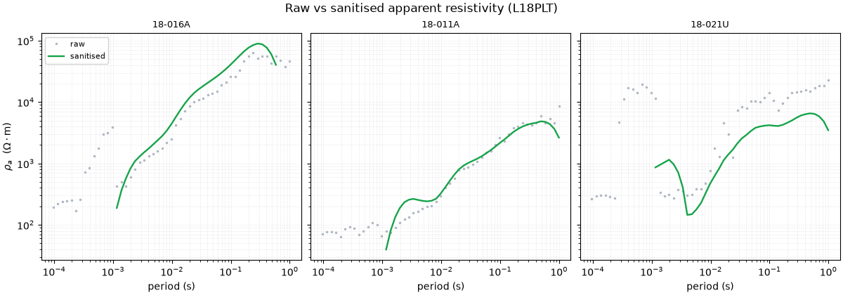
The payoff — three stations, raw against fully sanitised. The curves are trimmed to the trustworthy band, denoised, de-shifted, and rotated onto strike: inversion-ready.
raw_rho = curves(raw, "rho")
fin_rho = curves(final, "rho")
pick = [stations[3], stations[len(stations) // 2], stations[-4]]
plot_before_after(
    raw_rho,
    fin_rho,
    pick,
    quantity="rho",
    labels=("raw", "sanitised"),
    colors=("#b0b7c3", "#16a34a"),
    title="Raw vs sanitised apparent resistivity (L18PLT)",
)
<Figure size 1200x420 with 3 Axes>
Coverage after cleaning#
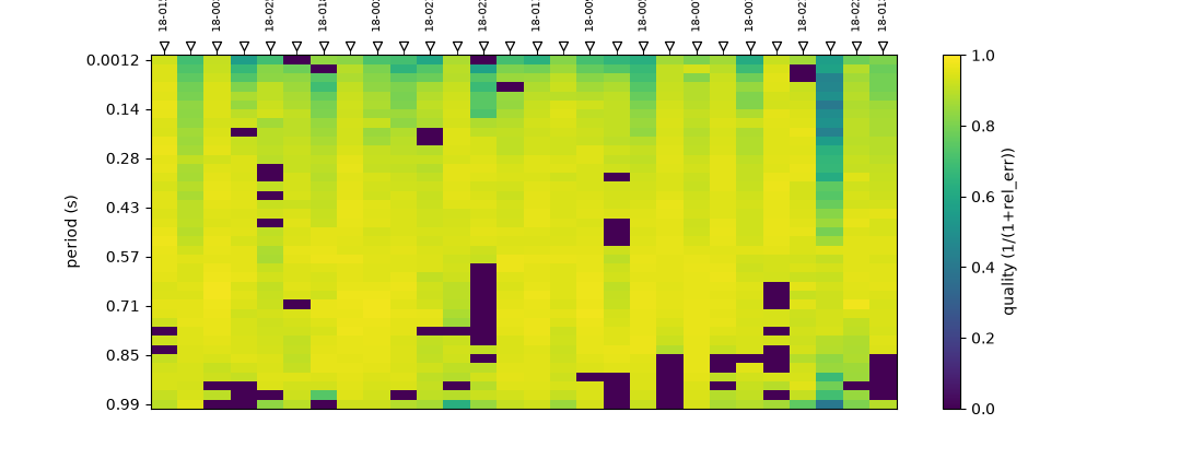
The same coverage map on the final data — trimmed to the coherent, high-quality core the editing kept.
plot_coverage_quality_heatmap(final, figsize=(11, 4.2))
<Axes: xlabel='Station', ylabel='period (s)'>
Write the sanitised EDIs#
write_sites() serialises the final Sites back
to standard EDI files — one per station, ready to archive, share, or hand
to an inversion. This is the real deliverable of a processing run.
import tempfile
from pathlib import Path

outdir = Path(tempfile.mkdtemp(prefix="sanitised_L18_"))
paths = write_sites(final, outdir, exist_ok=True)
print(f"wrote {len(paths)} sanitised EDIs, e.g. {[p.name for p in paths[:3]]}")

# round-trip: the output is real, re-loadable EDI data
from pycsamt.emtools._core import ensure_sites

reloaded = ensure_sites(str(outdir))
print(
    f"re-loaded {len(n_freq(reloaded))} EDIs, "
    f"{n_freq(reloaded).min()}-{n_freq(reloaded).max()} frequencies each"
)
wrote 28 sanitised EDIs, e.g. ['18-001A.edi', '18-002U.edi', '18-003A.edi']
re-loaded 28 EDIs, 25-39 frequencies each
The identical chain on a second line (L22PLT)#
Because every step is just Sites -> Sites, the whole workflow is a
reusable function. Applying it to L22PLT — a different line, same survey —
and writing its EDIs shows the processing generalises unchanged.
def sanitise(sites):
    s = drop_duplicates(sites, recursive=False)
    s = select_band(s, fmin=1e-3, fmax=1e3, recursive=False)
    s = drop_low_confidence_frequencies(s, threshold=0.5, recursive=False)
    s = notch_powerline(s, recursive=False)
    s = smooth_logfreq(s, win=5, recursive=False)
    s = correct_ss_ama(s, recursive=False)
    return rotate_to_strike(s, recursive=False)


raw22 = demo_line("L22PLT")
final22 = sanitise(raw22)
out22 = Path(tempfile.mkdtemp(prefix="sanitised_L22_"))
paths22 = write_sites(final22, out22, exist_ok=True)
print(
    f"L22PLT: {len(n_freq(raw22))} stations, "
    f"{n_freq(raw22).max()} raw -> {n_freq(final22).max()} sanitised "
    f"frequencies; wrote {len(paths22)} EDIs"
)
L22PLT: 25 stations, 53 raw -> 39 sanitised frequencies; wrote 25 EDIs
Takeaway. Processing in pyCSAMT is a chain of pure Sites -> Sites
steps: trim the frequency axis, condition the survivors, then write
sanitised EDIs. Every intermediate is a real, inspectable dataset, and the
whole chain wraps into a one-line sanitise() you can run on any line —
reproducible, auditable, and inversion-ready.
Total running time of the script: (0 minutes 3.708 seconds)