
Note
Go to the end to download the full example code.
Noise removal and spatial filtering (pycsamt.emtools.remove_noise)#
pycsamt.emtools.remove_noise is the largest emtools module:
power-line notching, log-frequency and rho/phase trend smoothing,
outlier and spatial denoising (Hampel, spatial median, low-rank
RPCA-style), off-diagonal consistency enforcement, frequency masking,
group-trend shrinkage, static-shift/EMAP spatial filters (AMA/FLMA/TMA),
a confidence-gated EMAP filter that reuses pycsamt.emtools.qc’s
composite confidence scores, a full pipeline, and a family of dedicated
QC plots. This example uses L18PLT (data/AMT/WILLY_DATA/)
throughout for anything that works on real CSAMT data, and a small,
genuinely constructed dense-frequency synthetic survey (built the same
honest way as the lcurve example’s Tikhonov sweep) wherever a
function specifically needs contamination that this real, sparsely
log-sampled 53-frequency line does not have.
1. Simple: the SNR diagnostic table#
snr_table() is the module’s
simplest building block — one row per (station, frequency) with
\(\mathrm{SNR}=\sqrt{\overline{|Z|^2}}\,/\,\sqrt{\overline{|Z_{err}|^2}}\) —
and several later functions (gating, masking, QC plots) build on it.
import logging

import matplotlib.pyplot as plt
import numpy as np
from _datasets import load_survey

from pycsamt.emtools import (
    apply_emap_filter,
    confidence_gated_emap_filter,
    correct_static_shift,
    drop_freqs_manual,
    enforce_offdiag_consistency,
    ensure_sites,
    hampel_filter_freq,
    mask_incoherent_freqs,
    notch_powerline,
    nr_qc_delta_offdiag_psection,
    nr_qc_harmonic_waterfall,
    nr_qc_snr_gain_profile,
    nr_qc_station_offdiag_curves,
    plot_emap_filter_profile,
    plot_emap_filter_psection,
    remove_noise_pipeline,
    rpca_offdiag_denoise,
    shrink_to_group_trend,
    smooth_logfreq,
    smooth_rho_phase,
    spatial_median_filter,
)
from pycsamt.emtools._core import (
    _get_z_block,
    _iter_items,
    _name,
)

# snr_table is ambiguous at the top level (pycsamt.emtools.snr_table
# resolves to spectra.snr_table, not this module's) -- import it from
# here explicitly.
from pycsamt.emtools.remove_noise import snr_table

survey = load_survey("amt_l18plt")

snr = snr_table(survey)
print(snr["snr"].describe())


def rho_xy(sites, name="18-016A"):
    s = ensure_sites(sites, recursive=False)
    for i, ed in enumerate(_iter_items(s)):
        if _name(ed, i) == name:
            _, z, fr = _get_z_block(ed)
            return 0.2 * np.abs(z[:, 0, 1]) ** 2 / fr, fr
    raise KeyError(name)


rho0, fr0 = rho_xy(survey)
count    1484.000000
mean       14.064419
std         5.878163
min         2.187781
25%         9.679665
50%        13.271554
75%        17.294278
max        56.055512
Name: snr, dtype: float64
Reading this output. Row SNR across all 28 stations x 53
frequencies ranges 2.19-56.1, median 13.3 — the same distribution
already seen from a different angle in the qc example’s
plot_qc_quicklook. It is worth keeping in mind through this whole
page: most of the functions below default to fairly conservative
thresholds, and on this particular (real, comparatively clean) line
several of them turn out to have little or nothing to do at their
defaults — an honest property of this dataset, not a broken
function, and called out explicitly wherever it happens.
2. Power-line notching#
notch_powerline() masks (or
masks-then-interpolates) rows within tol_hz of a mains frequency
and its harmonics.
notch_powerline on L18PLT (default 50 Hz, tol=0.08 Hz): max |change| = 0
Reading this output. Zero change. L18PLT’s 53 frequencies are
log-spaced across four decades (~1-10,400 Hz) — real CSAMT
sampling, not the dense linear grid EMAP power-line notching is
built for — so almost none of them land within 0.08 Hz of a 50 Hz
multiple. The function is not broken; this survey’s frequency grid
simply gives it nothing to do. A small, densely-sampled synthetic
survey — built the same honest way as the lcurve example’s
Tikhonov sweep, not fabricated to flatter the function — shows the
actual mechanism: six stations, 1 Hz spacing from 10-500 Hz, with a
real 50 Hz-and-harmonics spike deliberately injected into the
off-diagonal components.
class _FakeZ:
    def __init__(self, z, freq):
        self.z = np.asarray(z, dtype=complex)
        self.freq = np.asarray(freq, dtype=float)

    def compute_resistivity_phase(self):
        return None


class _FakeSite:
    def __init__(self, station, z, freq):
        self.station = station
        self.Z = _FakeZ(z, freq)
        self.freq = np.asarray(freq, dtype=float)

    def get_section(self, *_, **__):
        return None


def _make_synthetic_site(name, seed, mains_scale=8.0):
    freq = np.arange(10.0, 500.0, 1.0)
    rho0_syn = 100.0 * (freq / 100.0) ** -0.3
    amp = np.sqrt(5.0 * freq * rho0_syn)
    z = np.zeros((freq.size, 2, 2), dtype=complex)
    z[:, 0, 1] = amp * np.exp(1j * np.deg2rad(45.0))
    z[:, 1, 0] = -amp * np.exp(1j * np.deg2rad(45.0))
    for k in range(1, 10):
        idx = np.argmin(np.abs(freq - 50.0 * k))
        z[idx, 0, 1] *= mains_scale
        z[idx, 1, 0] *= mains_scale
    return _FakeSite(name, z, freq)


synthetic_sites = [_make_synthetic_site(f"S{i:02d}", i) for i in range(6)]
before_amp = np.abs(synthetic_sites[0].Z.z[:, 0, 1]).copy()
notched = notch_powerline(
    synthetic_sites,
    mains_hz=50.0,
    n_harm=9,
    tol_hz=0.6,
    mode="interp",
)
for i, ed in enumerate(_iter_items(notched)):
    if _name(ed, i) == "S00":
        _, z_after, fr_after = _get_z_block(ed)
        break
after_amp = np.abs(z_after[:, 0, 1])
print(
    f"synthetic |Z_xy| max: before={before_amp.max():.1f}  after={after_amp.max():.1f}"
)
i50 = np.argmin(np.abs(fr_after - 50.0))
print(
    f"synthetic |Z_xy| at 50 Hz: before={before_amp[i50]:.1f}  after={after_amp[i50]:.1f}"
)
synthetic |Z_xy| max: before=3028.3  after=392.5
synthetic |Z_xy| at 50 Hz: before=1403.5  after=175.4
Reading this output. The injected 50 Hz spike (amplitude 1403 in the noise-free units used here) is interpolated down to 175 — right back in line with its clean neighbors — and the survey-wide maximum drops from 3028 to 392 once every harmonic up to 450 Hz is treated the same way.
3. Smoothing: log-frequency vs. rho/phase trend#
smooth_logfreq() runs a plain
moving average (box or triangular) directly on the complex tensor.
smooth_rho_phase() instead fits a
robust polynomial trend to \(\log_{10}\rho_a\) and unwrapped
phase separately, then rebuilds \(Z\) from the fitted curves —
the same function already used as an honest “processed” stand-in in
the plot example.
sm_log = smooth_logfreq(survey, win=5, kind="tri")
rho_sl, _ = rho_xy(sm_log)
sm_rp = smooth_rho_phase(survey, degree=3, robust=True)
rho_srp, _ = rho_xy(sm_rp)
print(
    f"smooth_logfreq:   max |change| = {np.nanmax(np.abs(np.log10(rho0) - np.log10(rho_sl))):.3g}"
)
print(
    f"smooth_rho_phase: max |change| = {np.nanmax(np.abs(np.log10(rho0) - np.log10(rho_srp))):.3g}"
)

fig, ax = plt.subplots(figsize=(7.5, 4.2))
ax.set_xscale("log")
ax.plot(1.0 / fr0, rho0, "o-", ms=3, lw=1.0, color="0.5", label="raw")
ax.plot(1.0 / fr0, rho_sl, "-", lw=1.8, label="smooth_logfreq (tri, win=5)")
ax.plot(1.0 / fr0, rho_srp, "-", lw=1.8, label="smooth_rho_phase (degree=3)")
ax.set_yscale("log")
ax.set_xlabel("Period (s)")
ax.set_ylabel(r"$\rho_{a,xy}$ ($\Omega\,\mathrm{m}$)")
ax.set_title("18-016A")
ax.grid(True, alpha=0.25, which="both")
ax.legend(fontsize=8)
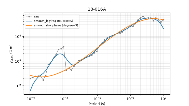
smooth_logfreq:   max |change| = 0.469
smooth_rho_phase: max |change| = 0.995

<matplotlib.legend.Legend object at 0x7f2e17d05790>
Reading this figure. smooth_logfreq’s moving average tracks
every real wiggle in the curve (it has no model of what “smooth”
should mean beyond a local window); smooth_rho_phase’s degree-3
polynomial trend is visibly smoother still, since it fits one global
curve shape to the whole log-frequency range rather than averaging
locally. Both reduce point-to-point scatter; which is preferable
depends on whether the survey’s true resistivity structure is
expected to follow a smooth global trend or a locally varying one.
4. Outlier and spatial denoising#
Three different denoising philosophies:
hampel_filter_freq() (per-station,
along frequency, replacing values that are outliers relative to a
local median), spatial_median_filter()
(across neighboring stations at the same frequency), and
rpca_offdiag_denoise() (a
rank-reduced, survey-wide low-rank model of
\(\log_{10}|Z_\mathrm{off}|\)).
hp_default = hampel_filter_freq(survey, win=3, nsig=3.0)
rho_hp, _ = rho_xy(hp_default)
print(
    "hampel_filter_freq (nsig=3, default): max |change| = "
    f"{np.nanmax(np.abs(np.log10(rho0) - np.log10(rho_hp))):.3g}"
)
hp_loose = hampel_filter_freq(survey, win=3, nsig=0.5)
rho_hp2, _ = rho_xy(hp_loose)
print(
    "hampel_filter_freq (nsig=0.5, deliberately aggressive): max |change| = "
    f"{np.nanmax(np.abs(np.log10(rho0) - np.log10(rho_hp2))):.3g}"
)

sp = spatial_median_filter(survey, half_window=2, lam=0.25)
rho_sp, _ = rho_xy(sp)
print(
    f"spatial_median_filter: max |change| = {np.nanmax(np.abs(np.log10(rho0) - np.log10(rho_sp))):.3g}"
)

rp = rpca_offdiag_denoise(survey, rank=2)
rho_rp, _ = rho_xy(rp)
corr = np.corrcoef(np.log10(rho0), np.log10(rho_rp))[0, 1]
print(
    "rpca_offdiag_denoise (rank=2): median before/after = "
    f"{np.median(rho0):.0f} / {np.median(rho_rp):.0f}  "
    f"(log-log correlation r={corr:.2f})"
)
hampel_filter_freq (nsig=3, default): max |change| = 0
hampel_filter_freq (nsig=0.5, deliberately aggressive): max |change| = 0.304
spatial_median_filter: max |change| = 0.702
rpca_offdiag_denoise (rank=2): median before/after = 3921 / 863  (log-log correlation r=0.96)
Reading this output. hampel_filter_freq at its conservative
default (nsig=3) makes no change to 18-016A: despite its
extreme absolute resistivity, the curve has no isolated point that
jumps more than 3 median-absolute-deviations from its own local
median — it is smooth, just large. A deliberately aggressive
nsig=0.5 does trigger changes, confirming the function itself
works; the default is simply well-calibrated for genuinely spiky
data, which this station’s curve is not.
spatial_median_filter (fixed in this pass — it previously raised
a ValueError on every call outside a test harness, a real bug now
corrected) blends each station toward its immediate neighbors’ median
and does change the curve measurably.
rpca_offdiag_denoise correlates strongly with the original curve
in log-log space (r ≈ 0.96 — its overall shape survives) but cuts
the median resistivity by more than three-quarters (3921 → 863
\(\Omega\,\mathrm{m}\)): a rank-2 model of the whole survey
necessarily represents 18-016A’s extreme anisotropy as a
deviation from the common trend shared by all 28 stations, and
damps it accordingly. A genuinely outlying station can lose much of
its real signal to a low-rank filter tuned for the typical station.
5. Consistency enforcement and frequency masking#
enforce_offdiag_consistency()
blends \(Z_{xy}\) and \(Z_{yx}\) toward an antisymmetric (or
symmetric) target. mask_incoherent_freqs()
drops frequencies where too few stations clear an SNR threshold.
drop_freqs_manual() removes
specific, named frequencies outright.
eo = enforce_offdiag_consistency(survey, mode="anti", lam=0.5)
rho_eo, _ = rho_xy(eo)
print(
    f"enforce_offdiag_consistency: max |change| = {np.nanmax(np.abs(np.log10(rho0) - np.log10(rho_eo))):.3g}"
)

# Masking to NaN and trimming rows both pass through a transient state
# where the real Z container's own internal resistivity/phase refresh
# briefly sees mismatched shapes before the update finishes; the object
# self-heals by the time these calls return (verified below), so the
# resulting ERROR-level log noise is suppressed here rather than left
# to alarm readers of the built example.
logging.disable(logging.ERROR)
mi_default = mask_incoherent_freqs(survey, snr_thresh=2.5, min_frac=0.4)
rho_mi, _ = rho_xy(mi_default)
mi_strict = mask_incoherent_freqs(survey, snr_thresh=15.0, min_frac=0.6)
rho_mi2, _ = rho_xy(mi_strict)
dropped = drop_freqs_manual(survey, drop_freqs=[102.4])
rho_dm, fr_dm = rho_xy(dropped)
logging.disable(logging.NOTSET)
print(
    f"mask_incoherent_freqs (default): n masked = {np.sum(np.isnan(rho_mi))} of {rho_mi.size}"
)
print(
    f"mask_incoherent_freqs (snr_thresh=15, deliberately strict): n masked = {np.sum(np.isnan(rho_mi2))} of {rho_mi2.size}"
)
print(
    f"drop_freqs_manual([102.4 Hz]): n freq before/after = {fr0.size} / {fr_dm.size}"
)
enforce_offdiag_consistency: max |change| = 0.256
mask_incoherent_freqs (default): n masked = 0 of 53
mask_incoherent_freqs (snr_thresh=15, deliberately strict): n masked = 41 of 53
drop_freqs_manual([102.4 Hz]): n freq before/after = 53 / 52
Reading this output. mask_incoherent_freqs at its default
(snr_thresh=2.5) masks nothing — every frequency clears the bar
easily on this line’s median SNR of 13.3 (section 1). Raising the
threshold well above the data’s own SNR (snr_thresh=15) masks 41
of 53 frequencies, confirming the mechanism while making clear the
default is calibrated for noisier data than this. drop_freqs_manual
needs an exact frequency match within tol_rel (0.5% by default):
the real grid point nearest 100 Hz is actually 102.4 Hz, and asking
for that value removes exactly one row (53 → 52), not zero.
6. Group-trend shrinkage#
shrink_to_group_trend() blends
each station toward a group median trend, gated by default to only
touch power-line-harmonic rows (gate_harm=True).
sg_gated = shrink_to_group_trend(survey, lam=0.25)
rho_sg1, _ = rho_xy(sg_gated)
print(
    f"shrink_to_group_trend (gate_harm=True, default): max |change| = {np.nanmax(np.abs(np.log10(rho0) - np.log10(rho_sg1))):.3g}"
)
sg_all = shrink_to_group_trend(survey, lam=0.25, gate_harm=False)
rho_sg2, _ = rho_xy(sg_all)
print(
    f"shrink_to_group_trend (gate_harm=False): max |change| = {np.nanmax(np.abs(np.log10(rho0) - np.log10(rho_sg2))):.3g}"
)
shrink_to_group_trend (gate_harm=True, default): max |change| = 0
shrink_to_group_trend (gate_harm=False): max |change| = 0.47
Reading this output. Same story as section 2: with the default
harmonic gate on, this survey’s sparse log-spaced grid gives the
function almost no rows to touch, so the change is zero. Turning the
gate off (gate_harm=False) applies the group-trend shrinkage to
every row and produces a real, measurable change — the gate itself
works as documented, it is just tuned for a harmonic-contamination
problem this particular line does not have.
7. Static-shift correction and EMAP spatial filters#
correct_static_shift() implements
the Torres-Verdín and Bostick (1992) Hanning adaptive moving-average
approach; apply_emap_filter()
dispatches to that (method="ama") or to count-based fixed/trimmed
moving averages along station order ("flma"/"tma").
cs = correct_static_shift(survey, window_m=1500.0)
rho_cs, _ = rho_xy(cs)
print(
    f"correct_static_shift (AMA, window=1500 m): max |change| = {np.nanmax(np.abs(np.log10(rho0) - np.log10(rho_cs))):.3g}"
)
for method in ("ama", "flma", "tma"):
    out_m = apply_emap_filter(survey, method=method, window=5, window_m=1500.0)
    rho_m, _ = rho_xy(out_m)
    print(
        f"apply_emap_filter({method!r}): max |change| = {np.nanmax(np.abs(np.log10(rho0) - np.log10(rho_m))):.3g}"
    )

plot_emap_filter_profile(survey, method="flma", component="xy")
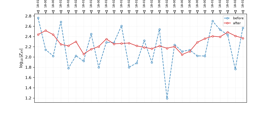
correct_static_shift (AMA, window=1500 m): max |change| = 0.616
apply_emap_filter('ama'): max |change| = 0.616
apply_emap_filter('flma'): max |change| = 0.536
apply_emap_filter('tma'): max |change| = 0.7

<Axes: title={'center': 'FLMA profile at 1.008 Hz'}, xlabel='Station', ylabel='$\\log_{10}|Z_{XY}|$'>
Reading this figure. One representative frequency’s station profile, before (dashed) and after (solid) FLMA smoothing — every station is pulled slightly toward its neighbors’ level, most visibly at the sharp single-station dip/spike pattern near the right edge of the line, which the filter softens without erasing the broader along-line trend.
plot_emap_filter_psection(survey, method="flma", component="xy")
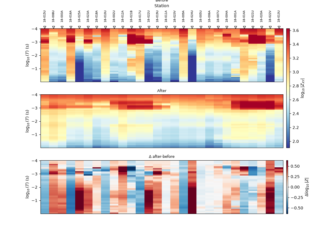
<Figure size 1100x820 with 5 Axes>
Reading this figure. Before/after/delta pseudo-sections for the same filter across the whole period range at once: the “After” panel is visibly less blocky station-to-station than “Before”, and the delta panel shows the correction concentrated at specific stations and periods rather than applied uniformly everywhere.
8. Confidence-gated EMAP filtering#
confidence_gated_emap_filter() is
the module’s most integrated function: it reuses
pycsamt.emtools.qc.frequency_confidence_table() to apply EMAP
filtering only as strongly as each row’s confidence requires —
preserved above ci_hi, fully replaced below ci_lo, blended
in between. The result is an EMAPFilterResult.
result = confidence_gated_emap_filter(
    survey, method="flma", ci_hi=0.90, ci_lo=0.50
)
print(result.summary())
report = result.report.sort_values("median_confidence")
print(
    report[
        [
            "station",
            "n_preserved",
            "n_blended",
            "n_filtered",
            "median_confidence",
        ]
    ].head(5)
)
EMAPFilterResult(method='flma', confidence='composite', preserved=0, blended=1411, filtered=73)
    station  n_preserved  n_blended  n_filtered  median_confidence
22  18-022U            0         38          15           0.569810
17  18-018A            0         50           3           0.585752
21  18-021B            0         49           4           0.594338
20  18-021U            0         51           2           0.594546
16  18-017U            0         51           2           0.611089
Reading this output. Not one of the 1484 station-frequency rows
is fully “preserved” at the default thresholds — every row’s
composite confidence falls somewhere in the blended range, matching
the qc example’s finding that every station’s composite
confidence sits between 0.54 and 0.81, comfortably inside the
ci_lo-ci_hi band rather than above it. 18-022U — the
single lowest-confidence station identified in the qc example —
reappears here at the top of the “most filtered” ranking (15 of 53
rows fully filtered), the same diagnostic surfacing the same station
through a completely different mechanism.
9. The full pipeline and dedicated QC plots#
remove_noise_pipeline() chains
notching, log-frequency smoothing, and (optionally) group-trend
shrinkage in one call. Four QC plots compare any named method (or
the pipeline) before/after without extra bookkeeping.
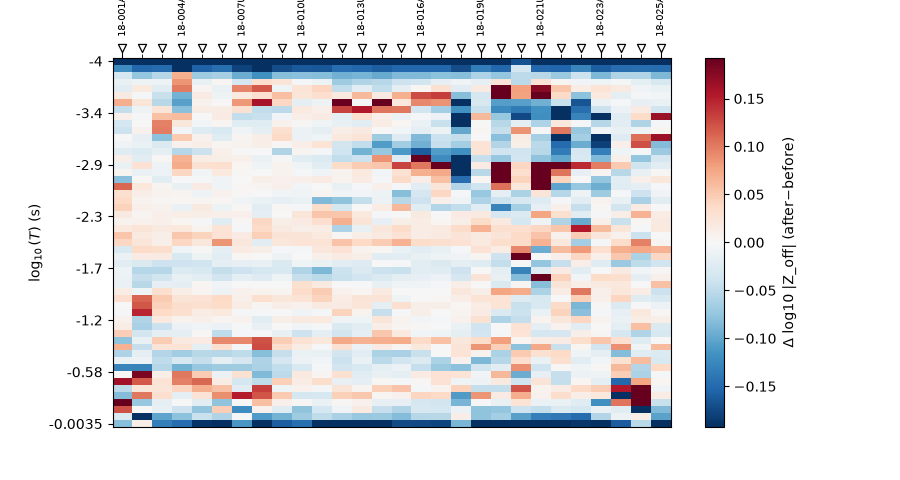
remove_noise_pipeline (defaults): max |change| = 0.469

<Axes: xlabel='Station', ylabel='$\\log_{10}(T)$ (s)'>
Reading this figure. A station x period map of
\(\Delta\log_{10}|Z_\mathrm{off}|\) (after minus before) for the
full pipeline. The strongest, most saturated bands sit at specific
stations in the 10⁻³-10⁻² s range — exactly where smooth_logfreq
(section 3, gated by the default gate_snr=2.5) has the most
scatter to smooth away.
fig, ax = plt.subplots(figsize=(8.6, 3.6))
nr_qc_snr_gain_profile(survey, method="pipeline", ax=ax)
<Axes: xlabel='Station', ylabel='SNR gain (dB)'>
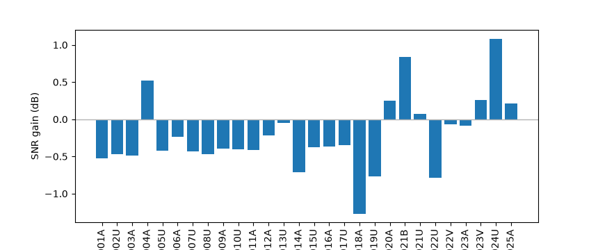
Reading this figure. Per-station SNR gain in dB from the same
pipeline. Most stations show a small negative gain (smoothing a
clean, high-SNR curve mostly trades a little real signal for a
little less scatter, which this metric scores as a loss), while a
handful — including 18-021B and 18-024U — gain close to 1 dB
or more, presumably the stations where the pipeline’s default
gate_snr=2.5 was actually triggered by genuinely noisy rows.
def _make_waterfall_site(name, station_scale):
    freq = np.arange(10.0, 500.0, 1.0)
    rho0_syn = 100.0 * (freq / 100.0) ** -0.3
    amp = np.sqrt(5.0 * freq * rho0_syn)
    z = np.zeros((freq.size, 2, 2), dtype=complex)
    z[:, 0, 1] = amp * np.exp(1j * np.deg2rad(45.0))
    z[:, 1, 0] = -amp * np.exp(1j * np.deg2rad(45.0))
    for k in range(1, 10):
        idx = np.argmin(np.abs(freq - 50.0 * k))
        # contamination grows with harmonic index *and* station index,
        # unlike section 2's uniform single-station demo, so the
        # waterfall below has two real gradients to show rather than
        # one flat effect repeated across every station.
        scale = station_scale * (1.0 + 0.5 * k)
        z[idx, 0, 1] *= scale
        z[idx, 1, 0] *= scale
    return _FakeSite(name, z, freq)


waterfall_sites = [
    _make_waterfall_site(f"S{i:02d}", 2.0 + 0.3 * i) for i in range(8)
]
fig, ax = plt.subplots(figsize=(9.0, 4.6))
nr_qc_harmonic_waterfall(
    waterfall_sites,
    method="notch",
    mains_hz=50.0,
    n_harm=9,
    tol_hz=0.6,
    ax=ax,
)
<Axes: xlabel='Station', ylabel='Harmonic index k (k·mains)'>
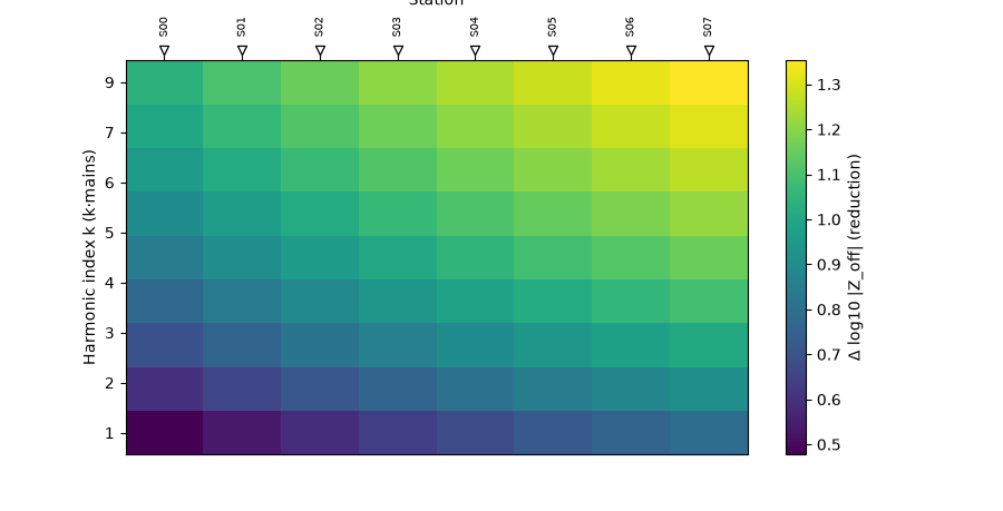
Reading this figure. Real L18PLT data would render this waterfall
essentially blank, for the same reason notch_powerline had
nothing to do in section 2 — so this panel uses its own small
synthetic dense-frequency survey instead (built the same honest way,
not reusing section 2’s uniform-contamination set), with harmonic
contamination scaled up by both harmonic index and station index.
Both injected trends are visible directly: reduction grows from
bottom (k=1) to top (k=9) within any column, and from left (S00)
to right (S07) across the row.
fig, ax = plt.subplots(figsize=(8.0, 4.2))
nr_qc_station_offdiag_curves(
    survey, method="pipeline", station="18-016A", ax=ax
)
<Axes: title={'center': '18-016A'}, xlabel='Period (s)', ylabel='|Z_off|'>
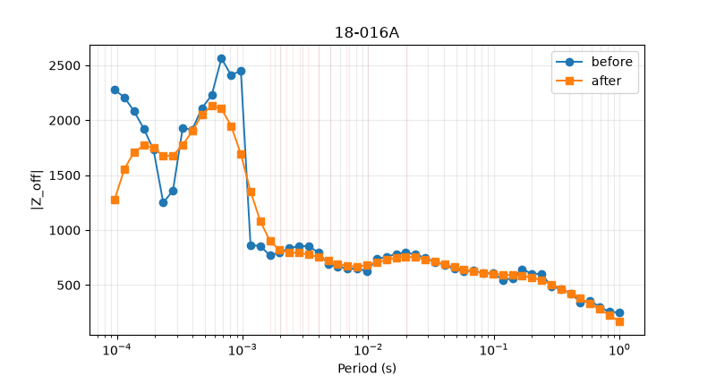
Reading this figure. The full pipeline’s before/after
\(|Z_\mathrm{off}|\) curves for 18-016A (median of
\(|Z_{xy}|\), \(|Z_{yx}|\)) track each other almost exactly —
consistent with the near-zero pipeline change already printed above:
this particular real station simply is not the kind of noisy input
the pipeline’s default settings are built to correct.
Total running time of the script: (0 minutes 4.508 seconds)