Apparent resistivity and phase

Apparent resistivity \(\rho_a\) and impedance phase are the most familiar MT/AMT data views. This example draws them straight from the impedance tensor of line L22PLT three ways: raw four-component station panels, cleaned component-coloured panels, and a single all-station overlay of the xy component.

The panel figures use pycsamt.emtools.plot.plot_raw_sites_1d() under a PYCSAMT_CONTROL context that sets the phase range and log/linear axis conventions; the overlay is built directly from Site.rho / Site.phase / Site.freq to show how little code the raw arrays need.

Raw four-component 1-D panels

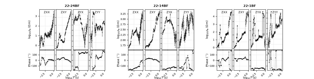
plot_raw_sites_1d() lays out apparent resistivity and phase for a handful of stations. With raw=True and all four tensor components (xx, xy, yx, yy), and a phase__range of ±180°, this is the unfiltered instrument view — useful for spotting bad components before any processing.

import matplotlib.pyplot as plt
from _datasets import load_sites

from pycsamt.api.control import PYCSAMT_CONTROL
from pycsamt.compat.matplotlib import get_cmap
from pycsamt.emtools._core import _iter_items, _name
from pycsamt.emtools.plot import plot_raw_sites_1d

L22 = load_sites("amt_l22plt")
panel_stations = ["22-1BF", "22-14BF", "22-24BF"]

with PYCSAMT_CONTROL.context(
    phase__range=(-180.0, 180.0),
    rho__view="log10",
    x__view="log10_period",
):
    plot_raw_sites_1d(
        L22,
        stations=panel_stations,
        components=("xx", "xy", "yx", "yy"),
        raw=True,
        ncols_groups=3,
        figsize_scale=(4.2, 3.2),
        show_component_legend=True,
    )

Component-coloured 1-D panels

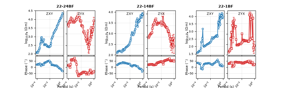
The same function with raw=False and the two principal off-diagonal components (xy, yx), a ±90° phase range and a linear period axis, gives the tidy, publication-style view of the same three stations.

with PYCSAMT_CONTROL.context(
    phase__range=(-90.0, 90.0),
    rho__view="log10",
    x__view="period",
):
    plot_raw_sites_1d(
        L22,
        stations=panel_stations,
        components=("xy", "yx"),
        raw=False,
        ncols_groups=3,
        figsize_scale=(3.2, 3.0),
        show_component_legend=True,
    )

All-station ρa / φ overlay (XY component)

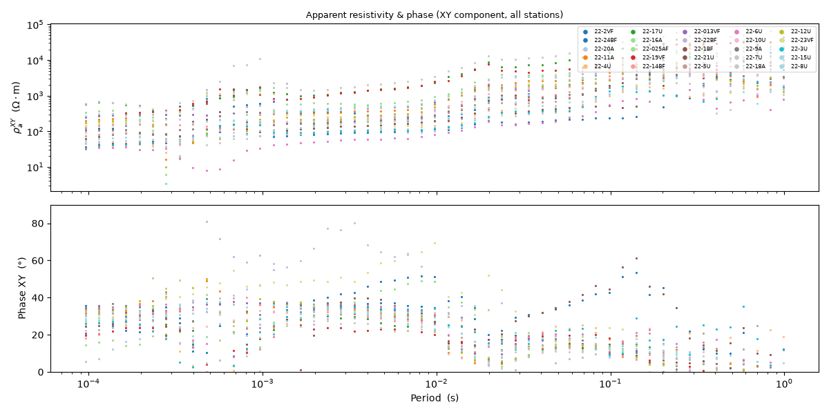
The plotting helpers are convenient, but the underlying arrays are right there on each Site. This overlay loops over all 25 stations and reads Site.rho / Site.phase / Site.freq directly — the xy apparent resistivity (top) and phase (bottom) versus period, one colour per station, showing the line’s overall dynamic range and consistency in a single figure.

sites = list(_iter_items(L22))
cmap = get_cmap("tab20", lut=len(sites))

fig, (ax_r, ax_p) = plt.subplots(2, 1, figsize=(12, 6), sharex=True)
for k, ed in enumerate(sites):
    per = 1.0 / ed.freq
    col = cmap(k)
    ax_r.loglog(
        per, ed.rho[:, 0, 1], ".", ms=2.5, color=col, label=_name(ed, k)
    )
    ax_p.semilogx(per, ed.phase[:, 0, 1], ".", ms=2.5, color=col)

ax_r.set_ylabel(r"$\rho_a^{XY}$  ($\Omega\cdot$m)")
ax_r.set_title(
    "Apparent resistivity & phase (XY component, all stations)",
    fontsize=9,
    pad=6,
)
ax_r.legend(
    ncol=5, fontsize=5.5, loc="upper right", markerscale=3, framealpha=0.7
)
ax_p.set_ylabel("Phase XY  (°)")
ax_p.set_xlabel("Period  (s)")
ax_p.set_ylim(0, 90)
fig.tight_layout()