Hydro interpretation: aquifer zones

HydroInterpreter is the qualitative hydrogeology step: it labels every cell of the section as a hydrogeological unit (overburden, aquifer, clay/aquitard, resistive basement) from resistivity thresholds, then groups the aquifer cells into connected zones you can hand to a driller. This example maps those units and zones on the synthetic section.

Fit the interpreter

The thresholds encode the conceptual model: the water table sits near 20 m, aquifer resistivity lies in 30-300 Ohm-m, and anything below clay_max is clay. fit classifies every sounding.

from _interp_data import demo_model

from pycsamt.interp import HydroInterpreter

# Use the unit-map figure (1st) as the card thumbnail.

rm = demo_model()
hydro = HydroInterpreter(
    water_table_depth=20.0,
    aquifer_range=(30.0, 300.0),
    clay_max=20.0,
    min_zone_thickness=8.0,
).fit(rm)

zones = hydro.aquifer_zones()
print(f"unit map: {hydro.unit_map.shape},  {len(zones)} aquifer zones found")
for z in zones[:3]:
    print(" ", z)

unit map: (34, 44),  44 aquifer zones found
  AquiferZone(station='S00', x=0.0, top=18.40909090909091, bottom=89.92424242424242, mean_rho_ohm_m=39.82536728080008, confidence=0.6226641892106022, zone_type='aquifer', metadata={})
  AquiferZone(station='S01', x=46.51162790697674, top=18.40909090909091, bottom=89.92424242424242, mean_rho_ohm_m=40.3071833422279, confidence=0.627422392137336, zone_type='aquifer', metadata={})
  AquiferZone(station='S02', x=93.02325581395348, top=18.40909090909091, bottom=89.92424242424242, mean_rho_ohm_m=39.51954693095646, confidence=0.6192355751894841, zone_type='aquifer', metadata={})

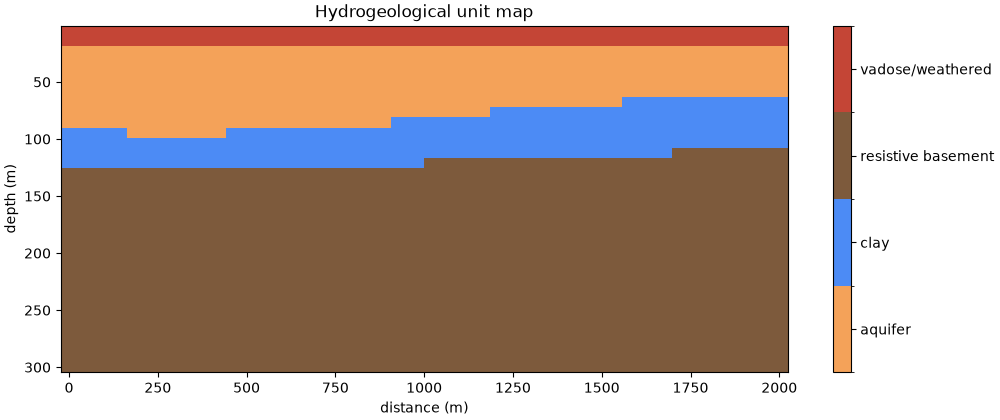
The hydrogeological unit map

unit_map is a (n_z, n_x) array of unit labels. Rendering it as a categorical image gives the interpreted section — the qualitative counterpart to the raw resistivity image in The resistivity model.

import matplotlib.pyplot as plt
import numpy as np
from matplotlib.colors import BoundaryNorm, ListedColormap

units = hydro.unit_map
names = sorted(np.unique(units))
code = {n: i for i, n in enumerate(names)}
coded = np.vectorize(code.get)(units)
palette = ["#f4a259", "#4c8bf5", "#7d5a3c", "#c44536", "#9aa0a6"][
    : len(names)
]
cmap = ListedColormap(palette)

fig, ax = plt.subplots(figsize=(10, 4.2), constrained_layout=True)
im = ax.pcolormesh(
    rm.x_centers,
    rm.z_centers,
    coded,
    cmap=cmap,
    norm=BoundaryNorm(np.arange(len(names) + 1) - 0.5, cmap.N),
    shading="auto",
)
ax.invert_yaxis()
ax.set_xlabel("distance (m)")
ax.set_ylabel("depth (m)")
ax.set_title("Hydrogeological unit map")
cb = fig.colorbar(im, ax=ax, ticks=range(len(names)))
cb.ax.set_yticklabels(names)

[Text(1, 0, 'aquifer'), Text(1, 1, 'clay'), Text(1, 2, 'resistive basement'), Text(1, 3, 'vadose/weathered')]

Station summary

station_summary() collapses the map to one row per station — its position, how many aquifer cells it holds, the number of zones, and a mean confidence — the table you would tabulate in a report.

summary = hydro.station_summary()
print(
    f"{'station':>8} {'x_m':>7} {'aquifer_cells':>14} {'n_zones':>8} "
    f"{'confidence':>11}"
)
for row in summary[:6]:
    print(
        f"{row['station']:>8} {row['x_m']:7.0f} {row['aquifer_cells']:14d} "
        f"{row['n_zones']:8d} {row['mean_confidence']:11.2f}"
    )

station     x_m  aquifer_cells  n_zones  confidence
    S00       0              8        1        0.51
    S01      47              8        1        0.51
    S02      93              8        1        0.51
    S03     140              8        1        0.51
    S04     186              9        1        0.50
    S05     233              9        1        0.50

Reading it. The unit map recovers a continuous aquifer beneath the overburden, pinching against the clay aquitard, over resistive basement — and the aquifer zones give its lateral extent directly. The next example turns these qualitative units into quantitative aquifer properties.