1-D layered models and geology priors

Everything in pycsamt.forward starts from a model: a stack of horizontal layers, each with a resistivity and (except the basal half-space) a thickness. LayeredModel is that container, and plot_model_1d() draws it as a resistivity-versus-depth staircase. This first example builds a small library of geologically-motivated models and shows three ways to look at them — one model, several overlaid, and random draws from the built-in GEOLOGY_PRIORS. The same model objects feed the sounding, 2-D, and 3-D examples that follow.

A small library of layered models

Each LayeredModel takes a list of layer resistivities (Ohm-m) and one fewer thickness (m); the last resistivity is the terminating half-space. These five span the common end-members: a conductive sedimentary sequence, a resistive crystalline basement, a geothermal profile with a shallow conductive clay cap, a uniform half-space, and a buried conductive layer.

from pycsamt.forward import LayeredModel, plot_model_1d

M_SEDIMENTARY = LayeredModel(
    [1_000.0, 20.0, 5.0, 300.0], [200.0, 600.0, 1_500.0], name="sedimentary"
)
M_CRYSTALLINE = LayeredModel(
    [800.0, 8_000.0, 600.0], [2_000.0, 15_000.0], name="crystalline"
)
M_GEOTHERMAL = LayeredModel(
    [500.0, 8.0, 250.0, 3_000.0], [100.0, 400.0, 2_500.0], name="geothermal"
)
M_HALFSPACE = LayeredModel([100.0], [], name="halfspace")
M_CONDUCTIVE = LayeredModel(
    [200.0, 5.0, 400.0, 100.0],
    [150.0, 500.0, 2_000.0],
    name="conductive-layer",
)

1. A single model as a depth profile

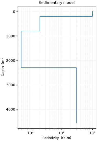
plot_model_1d() plots resistivity against depth on a log-resistivity axis. The sedimentary model’s conductive middle layers (20 and 5 Ohm-m) show up as the sharp low-resistivity step between ~200 m and ~800 m.

ax = plot_model_1d(M_SEDIMENTARY, title="Sedimentary model")

2. Several models overlaid

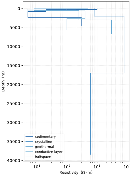
Passing a list of models (with labels) overlays them on one axis — the quickest way to compare how different geologies partition the subsurface. Note how the crystalline basement stays resistive with depth while the geothermal and conductive-layer models each carry a pronounced conductive interval.

ax = plot_model_1d(
    [M_SEDIMENTARY, M_CRYSTALLINE, M_GEOTHERMAL, M_CONDUCTIVE, M_HALFSPACE],
    labels=[
        "sedimentary",
        "crystalline",
        "geothermal",
        "conductive-layer",
        "halfspace",
    ],
    figsize=(4.5, 6),
)

3. Random draws from the geology priors

GEOLOGY_PRIORS defines plausible resistivity/thickness distributions for a set of named settings. LayeredModel.from_geology samples one realisation (fixed seed here for reproducibility) — the building block for generating synthetic training sets for the AI-inversion models.

rng_models, rng_labels = [], []
for scenario in (
    "sedimentary",
    "crystalline",
    "geothermal",
    "marine",
    "permafrost",
):
    m = LayeredModel.from_geology(scenario, seed=42)
    m.name = scenario
    rng_models.append(m)
    rng_labels.append(scenario)

ax = plot_model_1d(rng_models, labels=rng_labels, figsize=(4.5, 6))

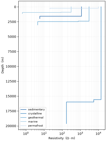
Reading this figure. Each curve is one random realisation of its named prior, so re-running with a different seed gives a different — but geologically consistent — profile. This is exactly how large synthetic datasets are assembled: sample thousands of models from the priors, run the forward solver on each (next examples), and train an inverse operator on the resulting (model, response) pairs.