Impedance phasor and determinant diagnostics

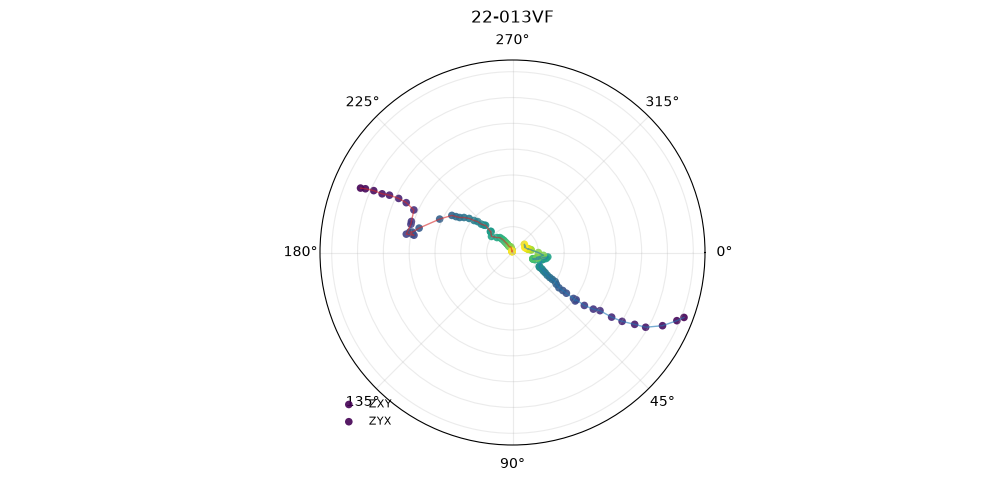
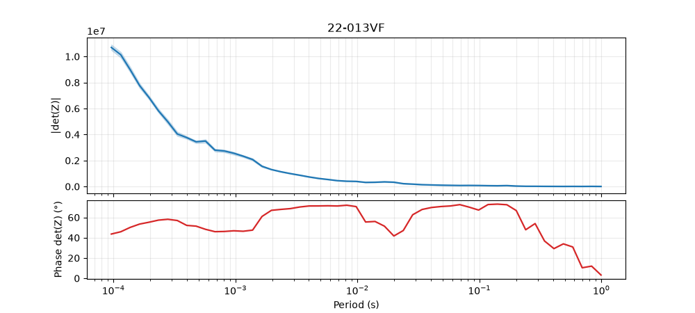
Two compact views of the impedance tensor itself, before any phase-tensor or dimensionality reduction. The phasor wheel shows the complex impedance components on the Argand plane; the determinant track follows the rotationally-invariant determinant impedance across period. Both are drawn for line L22PLT and both come from pycsamt.emtools.impedance.

Impedance phasor wheel

plot_phasor_wheel() plots the complex impedance components as phasors on the Argand plane, so the relative magnitude and phase of the xy and yx responses — and any departure from the ideal antidiagonal 2-D pattern — are visible directly.

from _datasets import load_sites

from pycsamt.emtools.impedance import (
    plot_determinant_track,
    plot_phasor_wheel,
)

L22 = load_sites("amt_l22plt")

plot_phasor_wheel(L22, figsize=(10, 5))

<PolarAxes: title={'center': '22-013VF'}>

Determinant impedance track

plot_determinant_track() follows the determinant impedance \(Z_{\det}=\sqrt{Z_{xx}Z_{yy}-Z_{xy}Z_{yx}}\) — a rotational invariant, and a common single-curve summary of a station’s response — across period for every station on the line.

plot_determinant_track(L22, figsize=(10, 4.5))

<Figure size 1000x450 with 2 Axes>