Draping a 2-D section over topography

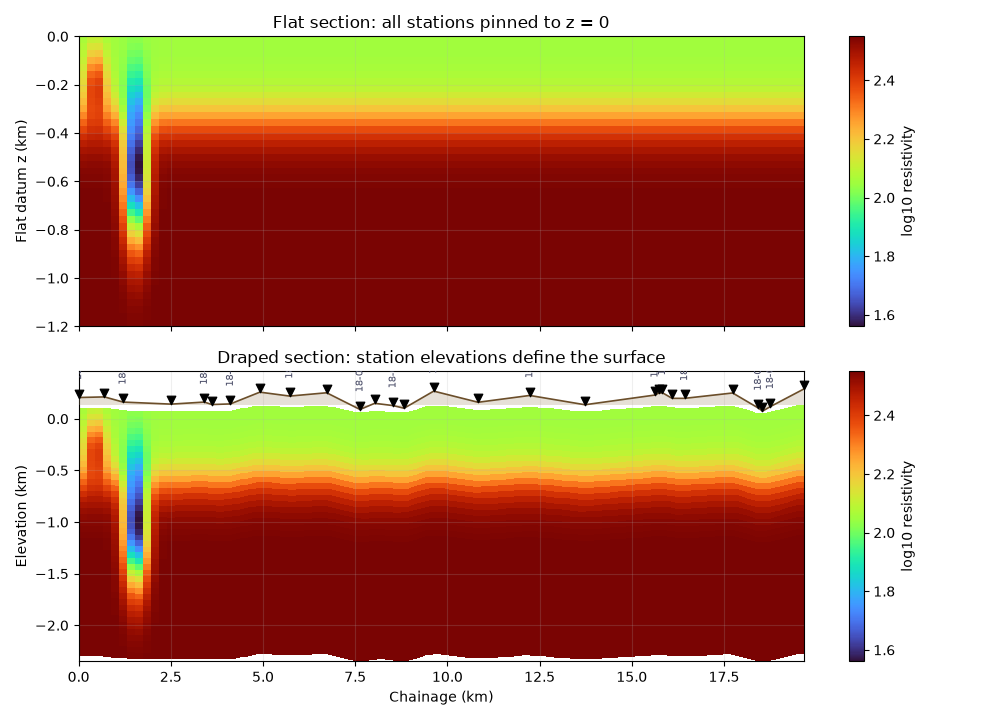
Depth sections are often built on a flat datum: x is profile distance and z is depth below zero. Real surveys have station elevations, so a section can be draped into an absolute-elevation frame.

This example answers:

How do I transform a flat 2-D section into terrain-following coordinates?

The resistivity model below is synthetic, but the station elevations are real WILLY L18PLT metadata.

import os
import sys
from pathlib import Path

import matplotlib.pyplot as plt
import numpy as np


def repo_root():
    root = os.environ.get("PYCSAMT_DOCS_REPO_ROOT")
    return Path(root) if root else Path(__file__).resolve().parents[3]


ROOT = repo_root()
if str(ROOT) not in sys.path:
    sys.path.insert(0, str(ROOT))

from pycsamt.emtools import ensure_sites
from pycsamt.topo import (
    TopoConfig,
    drape_section,
    draw_topo_section,
    extract_chainage,
    extract_elevation,
    extract_station_names,
    interp_elev,
)

sites = ensure_sites(
    ROOT / "data" / "AMT" / "WILLY_DATA" / "L18PLT", verbose=0
)
names = extract_station_names(sites)
chain_km = extract_chainage(sites)
elev_m = extract_elevation(sites)

1. Build a synthetic section on a flat depth grid

The data are log10 resistivity values. We create a conductive body beneath the middle of the line and a resistive near-surface cap, only to make the draping visible.

nx = 90
nz = 42
x_nodes = np.linspace(chain_km.min(), chain_km.max(), nx + 1)
z_nodes = np.linspace(0.0, 1.2, nz + 1)  # km, positive downward
x_centres = 0.5 * (x_nodes[:-1] + x_nodes[1:])
z_centres = 0.5 * (z_nodes[:-1] + z_nodes[1:])
X, Z = np.meshgrid(x_centres, z_centres)

log_rho = 2.3 + 0.25 * np.tanh((Z - 0.35) / 0.12)
log_rho -= 1.05 * np.exp(-((X - 1.55) ** 2 / 0.10 + (Z - 0.55) ** 2 / 0.08))
log_rho += 0.35 * np.exp(-((X - 0.45) ** 2 / 0.08 + (Z - 0.20) ** 2 / 0.02))

2. Compare flat and draped coordinates

elev_at_centres = interp_elev(chain_km, elev_m / 1000.0, x_centres)
x_draped, z_draped, log_rho_draped = drape_section(
    x_nodes,
    z_nodes,
    log_rho,
    elev_at_centres,
    exaggeration=2.0,
)

fig, axs = plt.subplots(2, 1, figsize=(10, 7.2), sharex=True)

pcm0 = axs[0].pcolormesh(
    x_nodes, -z_nodes, log_rho, shading="auto", cmap="turbo"
)
axs[0].set_ylabel("Flat datum z (km)")
axs[0].set_title("Flat section: all stations pinned to z = 0")
axs[0].grid(alpha=0.2)
fig.colorbar(pcm0, ax=axs[0], label="log10 resistivity")

pcm1 = axs[1].pcolormesh(
    x_draped, z_draped, log_rho_draped, shading="auto", cmap="turbo"
)
axs[1].set_xlabel("Chainage (km)")
axs[1].set_ylabel("Elevation (km)")
axs[1].set_title("Draped section: station elevations define the surface")
draw_topo_section(
    axs[1],
    chain_km,
    elev_m,
    names,
    cfg=TopoConfig(exaggeration=2.0, fill_alpha=0.28),
    dark=False,
)
axs[1].grid(alpha=0.2)
fig.colorbar(pcm1, ax=axs[1], label="log10 resistivity")
fig.tight_layout()

3. Why display exaggeration matters

In drape_section the physical surface elevation stays in kilometres above sea level, while the depth axis is stretched by the exaggeration factor. draw_topo_section can also exaggerate the rendered overlay. Always state the display exaggeration used in a figure.

for exaggeration in (1.0, 2.0, 4.0):
    _, z_tmp, _ = drape_section(
        x_nodes, z_nodes, log_rho, elev_at_centres, exaggeration=exaggeration
    )
    section_base = z_tmp[-1]
    print(
        f"exaggeration={exaggeration:g}: section-base elevation range "
        f"{section_base.min():.3f} to {section_base.max():.3f} km"
    )

exaggeration=1: section-base elevation range -1.150 to -1.066 km
exaggeration=2: section-base elevation range -2.350 to -2.266 km
exaggeration=4: section-base elevation range -4.750 to -4.666 km

The important rule is: use topography to place the model in a realistic elevation frame, but do not let display exaggeration masquerade as geology.