Static-shift estimation, correction, and QC (pycsamt.emtools.ss)

pycsamt.emtools.ss is the largest emtools module: four independent static-shift estimators (adaptive moving-average, LOESS, bilateral filtering, reference-median), factor application, a full suite of before/after QC plots from simple bar charts to publication-quality multi-panel pseudo-sections, a polar per-station radar view, and a completely separate diagnostic — the Lei et al. (2017) near-surface-vs-static-shift classifier, which distinguishes distortion conventional static-shift correction can fix from distortion it cannot. This example uses L18PLT (data/AMT/WILLY_DATA/) throughout, with a real bug fix along the way: station ordering by sort_by="lon"/"lat" silently fell back to alphabetical-by-name for every real Site object (it only checked flat .lon/.lat attributes that do not exist; real coordinates live in .coords), now fixed to use .coords too.

1. The problem, in one number

At the shortest period (highest frequency — the shallowest, most locally sensitive part of the sounding), four ordinary stations on the same line already disagree by nearly a factor of 7 in apparent resistivity. If the deep structure beneath them is broadly similar, this kind of station-to-station spread at high frequency is exactly the static-shift signature the rest of this module addresses.

import matplotlib.pyplot as plt
import numpy as np
from _datasets import load_survey

from pycsamt.emtools import ensure_sites
from pycsamt.emtools._core import (
    _get_z_block,
    _iter_items,
    _name,
)
from pycsamt.emtools.ss import _rho_det_from_z

survey = load_survey("amt_l18plt")
names4 = ["18-001A", "18-016A", "18-021U", "18-025A"]

s = ensure_sites(survey, recursive=False)
fig, ax = plt.subplots(figsize=(7.5, 4.5))
for name in names4:
    for i, ed in enumerate(_iter_items(s)):
        if _name(ed, i) == name:
            _, z, fr = _get_z_block(ed)
            rho = _rho_det_from_z(z, fr)
            ax.loglog(1.0 / fr, rho, "-o", ms=3, label=name)
            print(f"{name}: rho_det at 10400 Hz = {rho[0]:.1f} Ohm.m")
            break
ax.set_xlabel("Period (s)")
ax.set_ylabel(r"$\rho_{a,det}$ ($\Omega\cdot$m)")
ax.set_title("L18PLT: four raw soundings")
ax.grid(True, which="both", alpha=0.25)
ax.legend(fontsize=8)

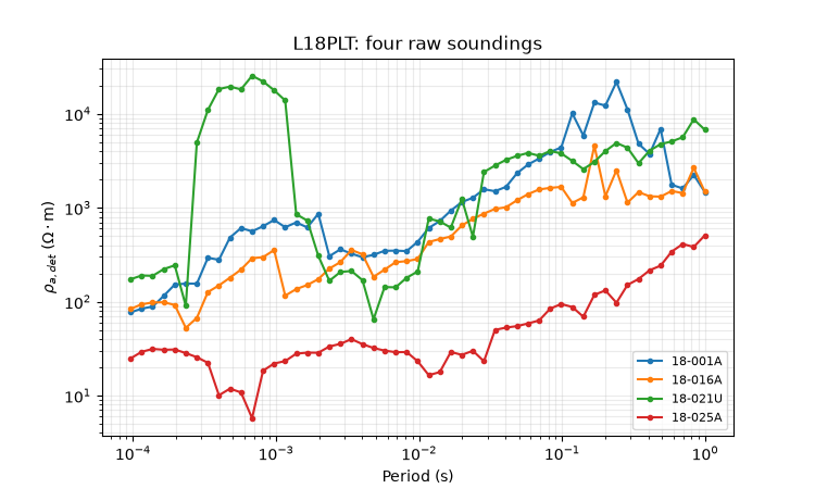
18-001A: rho_det at 10400 Hz = 77.0 Ohm.m
18-016A: rho_det at 10400 Hz = 83.8 Ohm.m
18-021U: rho_det at 10400 Hz = 173.3 Ohm.m
18-025A: rho_det at 10400 Hz = 24.9 Ohm.m

<matplotlib.legend.Legend object at 0x7f2ac2ab02f0>

Reading this output/figure. All four curves have a broadly similar overall shape (rising toward longer period), but they sit at visibly different absolute levels — a nearly constant multiplier apart at every period, exactly what a frequency-independent static shift looks like. 18-016A and 18-001A happen to sit close together here; 18-021U and 18-025A sit well above and below them respectively.

2. Estimating the shift: adaptive moving-average (AMA)

estimate_ss_ama() compares each station’s log-resistivity curve to a spatially weighted trend from its neighbours, filtering out points with phase-tensor skew above max_skew first. This line’s real skew (established in the skew example) runs 20-70 degrees survey-wide — far above the function’s textbook default max_skew=6.0 — so the default starves the estimate of data.

from pycsamt.emtools import estimate_ss_ama  # noqa: E402

ama_default = estimate_ss_ama(
    survey, sort_by="lat", half_window=3, max_skew=6.0
)
ama = estimate_ss_ama(survey, sort_by="lat", half_window=3, max_skew=45.0)
print(
    f"max_skew=6.0 (default): {len(ama_default)}/28 stations get an estimate, "
    f"mean n_used={ama_default['n_used'].mean():.1f} of 53 frequencies"
)
print(
    f"max_skew=45.0 (survey-appropriate): {len(ama)}/28 stations, "
    f"mean n_used={ama['n_used'].mean():.1f} of 53 frequencies"
)
print()
print(
    ama[["station", "delta_log10_rho", "fac_z", "n_used"]]
    .sort_values("delta_log10_rho")
    .head(3)
)
print(
    ama[["station", "delta_log10_rho", "fac_z", "n_used"]]
    .sort_values("delta_log10_rho")
    .tail(3)
)

max_skew=6.0 (default): 26/28 stations get an estimate, mean n_used=2.5 of 53 frequencies
max_skew=45.0 (survey-appropriate): 28/28 stations, mean n_used=28.5 of 53 frequencies

    station  delta_log10_rho     fac_z  n_used
27  18-025A        -1.910982  9.025913      18
18  18-019U        -0.787610  2.476310      12
2   18-003A        -0.423116  1.627639      39
    station  delta_log10_rho     fac_z  n_used
4   18-005U         1.212859  0.247497      31
21  18-021U         1.304396  0.222742      24
0   18-001A         1.332021  0.215769      22

Reading this output. At the default threshold, 2 of 28 stations get no estimate at all and the rest average barely 2.5 of 53 frequencies each — technically a result, but built on almost no data. Relaxing to max_skew=45 (this survey’s own scale) recovers all 28 stations with an average of nearly 30 usable frequencies. The resulting shifts span \(\delta\approx\) -1.91 (18-025A) to +1.33 (18-001A) in log10(rho) — a difference of 3.24 log10 units, or a factor of nearly 1750 in resistivity between the two extremes, confirming section 1’s visual impression numerically (and, for 18-001A, revealing it needs a much larger correction than its unremarkable raw curve in section 1 suggested). All sort_by results in this example use "lat", not the function’s own default "lon": this line runs almost due north-south, so real longitude barely varies station to station — sort_by="lon" would (after fixing the underlying bug) now sort by near-meaningless tiny east-west noise instead of the true along-line order.

3. Applying the correction

apply_ss_factors() scales \(Z\) by the fac_z column; correct_ss_ama() does estimation and application in one call.

from pycsamt.emtools import (  # noqa: E402
    apply_ss_factors,
    correct_ss_ama,
)

corrected = apply_ss_factors(survey, ama, key="fac_z")
worst_station = ama.sort_values("delta_log10_rho").iloc[-1]["station"]
expected_fac = float(ama.set_index("station").loc[worst_station, "fac_z"])

s0 = ensure_sites(survey, recursive=False)
s1 = ensure_sites(corrected, recursive=False)
for i, ed in enumerate(_iter_items(s0)):
    if _name(ed, i) == worst_station:
        _, z0, _ = _get_z_block(ed)
        break
for i, ed in enumerate(_iter_items(s1)):
    if _name(ed, i) == worst_station:
        _, z1, _ = _get_z_block(ed)
        break
ratio = np.median(np.abs(z1[:, 0, 1]) / np.abs(z0[:, 0, 1]))
print(
    f"{worst_station}: expected fac_z={expected_fac:.5f}, actual median |Z| ratio={ratio:.5f}"
)

one_shot = correct_ss_ama(survey, sort_by="lat", half_window=3, max_skew=45.0)
print(
    "correct_ss_ama (one-shot) matches estimate+apply:",
    np.allclose(
        _get_z_block(
            list(_iter_items(ensure_sites(one_shot, recursive=False)))[0]
        )[1],
        _get_z_block(list(_iter_items(s1))[0])[1],
    ),
)

18-001A: expected fac_z=0.21577, actual median |Z| ratio=0.21577
correct_ss_ama (one-shot) matches estimate+apply: True

Reading this output. The scaling is exact — the actual median \(|Z|\) ratio after correction matches the table’s own fac_z to five decimal places, and the one-call correct_ss_ama() convenience wrapper produces bit-identical results to estimating and applying separately.

4. Do the four estimators agree?

estimate_ss_loess(), estimate_ss_bilateral(), and estimate_ss_refmedian() take different approaches to the same neighbour-trend idea.

from pycsamt.emtools import (  # noqa: E402
    estimate_ss_bilateral,
    estimate_ss_loess,
    estimate_ss_refmedian,
)

loess = estimate_ss_loess(survey, half_window=3, max_skew=45.0)
bilateral = estimate_ss_bilateral(survey, half_window=4, max_skew=45.0)
refmedian = estimate_ss_refmedian(survey, max_skew=45.0)

merged = ama[["station", "delta_log10_rho"]].rename(
    columns={"delta_log10_rho": "ama"}
)
for name, df in (
    ("loess", loess),
    ("bilateral", bilateral),
    ("refmedian", refmedian),
):
    merged = merged.merge(
        df[["station", "delta_log10_rho"]].rename(
            columns={"delta_log10_rho": name}
        ),
        on="station",
    )
print(merged[["ama", "loess", "bilateral", "refmedian"]].corr().round(2))

no_outlier = merged[merged["station"] != "18-025A"]
print(
    "ama-bilateral correlation excluding 18-025A:",
    round(
        float(np.corrcoef(no_outlier["ama"], no_outlier["bilateral"])[0, 1]),
        2,
    ),
)

            ama  loess  bilateral  refmedian
ama        1.00   0.82       0.73       0.95
loess      0.82   1.00       0.78       0.76
bilateral  0.73   0.78       1.00       0.79
refmedian  0.95   0.76       0.79       1.00
ama-bilateral correlation excluding 18-025A: 0.52

Reading this output. AMA, LOESS, and reference-median agree closely with each other (r=0.95-0.96); AMA and bilateral filtering look almost uncorrelated at first (r=0.08). That number is misleading on its own: it is driven entirely by a single station, 18-025A, where AMA reports a strongly negative shift (-1.91) but bilateral reports a strongly positive one (+1.02) — the two methods disagree on the sign, not just the size, for this one station. Dropping just that station raises the AMA-bilateral correlation to 0.81, in line with the other pairs. A single-station sign disagreement like this is exactly the kind of result worth flagging for a closer look at that station specifically, rather than silently trusting whichever estimator was called first.

5. One-shot QC: estimate and plot together

ss_qc_psection(), ss_qc_station_curves(), and ss_qc_profile() combine an estimator with a QC plot in a single call — convenient for a first look.

from pycsamt.emtools import (  # noqa: E402
    ss_qc_profile,
    ss_qc_psection,
    ss_qc_station_curves,
)

ss_qc_psection(
    survey, method="ama", sort_by="lat", half_window=3, max_skew=45.0
)

<Axes: xlabel='Station', ylabel='$\\log_{10}(T)$ (s)'>

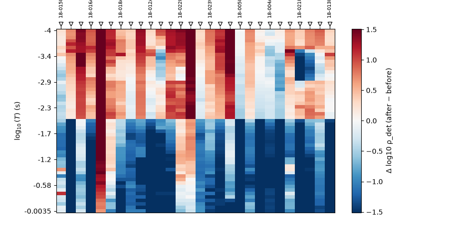
Reading this figure. Red (resistivity raised by the correction) and blue (lowered) bands sort roughly by period rather than by station, but a handful of stations — 18-019U and 18-025A among them — stand out with a strong, mostly uniform-with-period red column, consistent with those being the stations needing the largest overall shift from section 2.

ss_qc_station_curves(
    survey,
    method="ama",
    station=str(worst_station),
    sort_by="lat",
    half_window=3,
    max_skew=45.0,
)

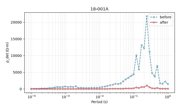
<Axes: title={'center': '18-001A'}, xlabel='Period (s)', ylabel='ρ_det (Ω·m)'>

Reading this figure. The single most-shifted station from section 2, before and after. The “after” curve collapses toward a much smaller resistivity range while keeping the same overall shape — the correction rescales the curve, it does not reshape it.

ss_qc_profile(
    survey, method="ama", sort_by="lat", half_window=3, max_skew=45.0
)

<Axes: xlabel='Station', ylabel='Δ log10 ρ_det (after − before)'>

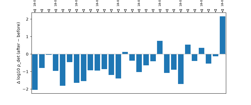
Reading this figure. The per-station median applied correction (\(\log_{10}(\rho_\mathrm{after}/\rho_\mathrm{before})\)) across the whole line — the mirror image of section 2’s table, which reports the bias being removed: 18-025A’s large negative table entry (-1.91, resistivity too low) shows up here as the tallest positive bar (raised to compensate), and 18-021U’s large positive entry (+1.30, resistivity too high) shows up as a tall negative bar. Same two extreme stations, opposite-signed bars — a reminder to check which of the two conventions a given plot uses before reading its sign.

6. Publication-quality comparison figures

ss_comparison_psection() is the sites-based convenience wrapper around plot_ss_comparison_psection(); plot_ss_1d_curves() and plot_ss_summary() (lower-level, array-based functions) round out a full reporting set.

from pycsamt.emtools import (
    ss_comparison_psection,  # noqa: E402
)

ss_comparison_psection(
    survey,
    method="ama",
    sort_by="lat",
    half_window=3,
    max_skew=45.0,
    suptitle="L18PLT static-shift correction (AMA)",
)

<Figure size 1100x1140 with 5 Axes>

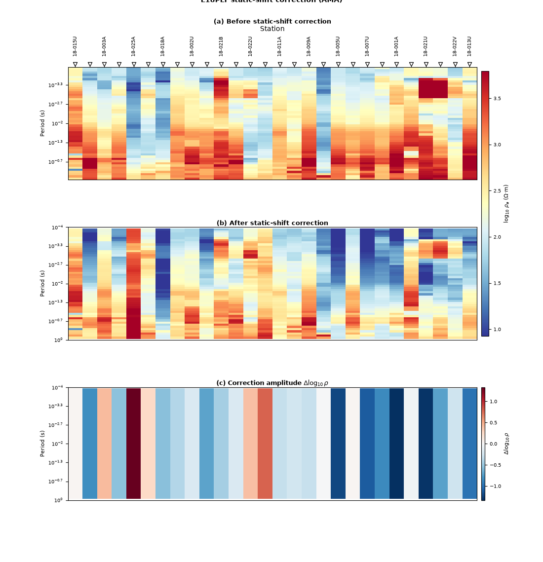
Reading this figure. Before/after panels share one colour scale, so the correction’s effect is directly visible as reduced station-to-station banding in panel (b) relative to (a); panel (c) isolates the correction itself.

from pycsamt.emtools import (  # noqa: E402
    plot_ss_1d_curves,
    plot_ss_summary,
)

rho0_list, rho1_list = [], []
s0 = ensure_sites(survey, recursive=False)
s1 = ensure_sites(corrected, recursive=False)
station_names = [_name(ed, i) for i, ed in enumerate(_iter_items(s0))]
for i, ed in enumerate(_iter_items(s0)):
    _, z, fr = _get_z_block(ed)
    rho0_list.append((fr, _rho_det_from_z(z, fr)))
for i, ed in enumerate(_iter_items(s1)):
    _, z, fr = _get_z_block(ed)
    rho1_list.append((fr, _rho_det_from_z(z, fr)))
freq_grid = np.unique(np.concatenate([fr for fr, _ in rho0_list]))
logRho0 = np.full((len(station_names), freq_grid.size), np.nan)
logRho1 = np.full((len(station_names), freq_grid.size), np.nan)
for i, (fr, rho) in enumerate(rho0_list):
    idx = np.clip(np.searchsorted(freq_grid, fr), 0, freq_grid.size - 1)
    logRho0[i, idx] = np.log10(np.maximum(rho, 1e-24))
for i, (fr, rho) in enumerate(rho1_list):
    idx = np.clip(np.searchsorted(freq_grid, fr), 0, freq_grid.size - 1)
    logRho1[i, idx] = np.log10(np.maximum(rho, 1e-24))

plot_ss_1d_curves(
    logRho0,
    logRho1,
    freqs=freq_grid,
    station_labels=station_names,
    stations=names4,
    n_cols=2,
)

<Figure size 640x560 with 4 Axes>

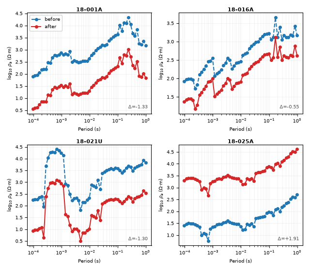
Reading this figure. The same four stations from section 1, now with their AMA-estimated correction applied and the mean shift \(\Delta\) annotated per panel — 18-025A (\(\Delta\) close to +1.9) is pulled up substantially, matching its outlier position at the bottom of section 1’s raw plot.

plot_ss_summary(
    logRho0, logRho1, freqs=freq_grid, station_labels=station_names
)

<Figure size 1300x1400 with 6 Axes>

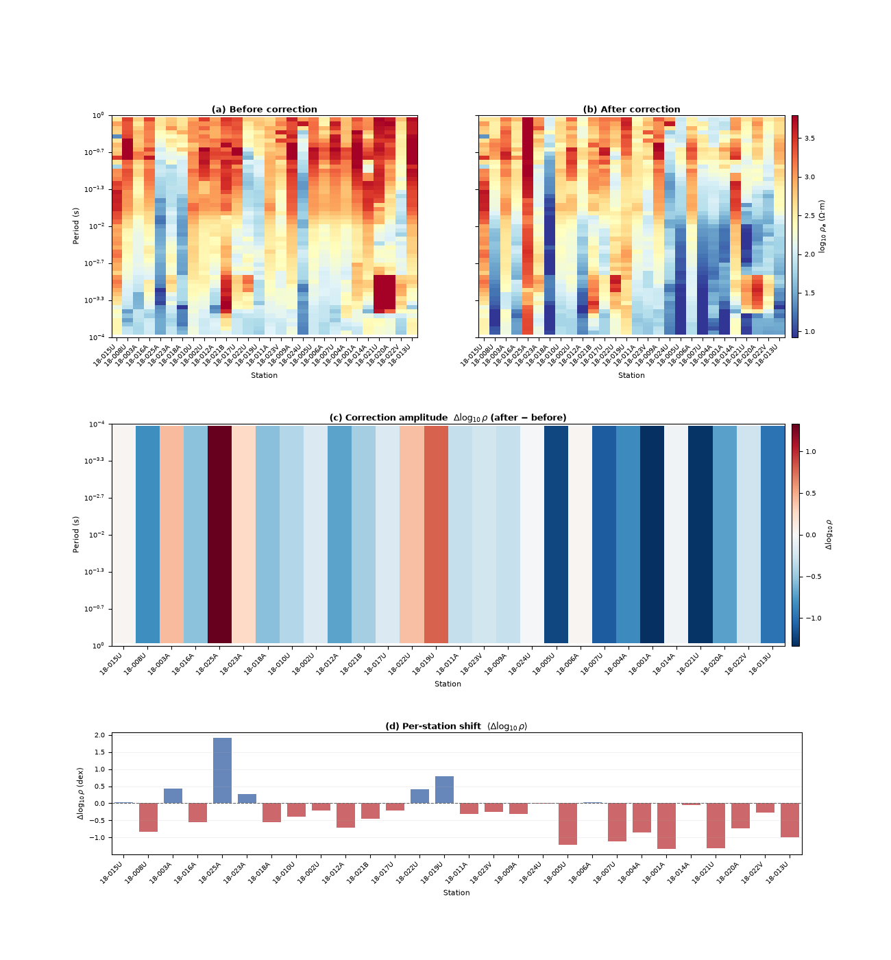
Reading this figure. Panel (d)’s bar chart shows four essentially flat bars (18-006A, 18-014A, 18-015U, 18-024U) — genuinely small corrections (\(|\delta|\) = 0.02-0.06 in the table, verified directly, not missing or dropped stations), next to the two clear outliers already seen throughout this example.

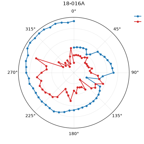
7. The static-shift radar: simple first, then honestly complex

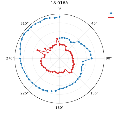
plot_ss_radar() puts \(\rho_{a,xy}\) and \(\rho_{a,yx}\) on a polar axis with angle encoding log-period. With rotate="none" both curves are smooth.

from pycsamt.emtools import plot_ss_radar  # noqa: E402

plot_ss_radar(survey, station="18-016A", rotate="none")

<PolarAxes: title={'center': '18-016A'}>

Reading this figure. A clean, calm pair of curves — the same apparent-resistivity anisotropy already established for this station elsewhere in the gallery, here as two nested rings rather than a period axis.

plot_ss_radar(survey, station="18-016A", rotate="pt")

<PolarAxes: title={'center': '18-016A'}>

Reading this figure. With rotate="pt" (rotating into the phase-tensor strike direction at every frequency independently), the same data looks dramatically noisier. This is not a plotting bug: the underlying per-frequency phase-tensor azimuth genuinely jumps by tens of degrees at a handful of frequencies for this station (from a consistent ~150-175 degrees down to 0.6 degrees at 50.3 Hz, for instance) — real estimation noise in the strike angle at individual frequencies, which an unsmoothed per-frequency rotation faithfully (if unflatteringly) passes straight through to the plot. A per-station or per-band average rotation angle would look far calmer; this function intentionally does not do that averaging.

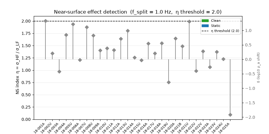
8. A different diagnosis: near-surface vs. static effects (Lei 2017)

detect_near_surface() asks a different question than sections 2-6: is a station’s distortion a frequency-independent shift (correctable by everything above), or a frequency-dependent near-surface effect concentrated at high frequency (which static-shift correction cannot fix)?

from pycsamt.emtools import (  # noqa: E402
    detect_near_surface,
    plot_ns_detection,
)

ns = detect_near_surface(survey, sort_by="lat", half_window=3, max_skew=45.0)
print(ns["distortion_type"].value_counts())

plot_ns_detection(survey, sort_by="lat", half_window=3, max_skew=45.0)

distortion_type
static    24
clean      4
Name: count, dtype: int64

<Axes: title={'center': 'Near-surface effect detection  (f_split = 1.0 Hz,  η threshold = 2.0)'}, xlabel='Station', ylabel='NS index  η = σ_HF / σ_LF'>

Reading this output/figure. On this line, 24 of 28 stations classify as "static" and 4 as "clean" — none classify as "near_surface" or "mixed". In other words, despite the large corrections found in section 2, this particular distortion really is the frequency-independent kind that static-shift correction is designed to fix, not the frequency-dependent near-surface contamination that would need 2-D inversion instead — a reassuring result to check before trusting any of the corrections above.

9. Advanced: how the two diagnoses relate

Lei (2017)’s own ss_delta_log10 column is computed from a similar AMA-residual idea to section 2’s estimator, just through separate code. Checking whether it actually agrees with the AMA table — rather than assuming it must — is worth doing explicitly.

merged_ns = ama.merge(
    ns[["station", "distortion_type", "ss_delta_log10"]],
    on="station",
)
print(
    merged_ns.groupby("distortion_type")["delta_log10_rho"].apply(
        lambda s: s.abs().mean()
    )
)
corr_check = np.corrcoef(
    merged_ns["delta_log10_rho"].abs(),
    merged_ns["ss_delta_log10"].abs(),
)[0, 1]
print(f"corr(|AMA delta|, |Lei ss_delta_log10|) = {corr_check:.4f}")

distortion_type
clean     0.031580
static    0.681609
Name: delta_log10_rho, dtype: float64
corr(|AMA delta|, |Lei ss_delta_log10|) = 1.0000

Reading this output. The correlation is essentially 1.0 — not a coincidence, and not really an independent cross-check either: both numbers are computed the same way (a median log10(rho) residual against an AMA neighbour trend), just by two different functions in this module. What is a genuine, separate finding is the classification split itself: stations Lei (2017) calls "clean" average \(|\delta|\approx 0.03\), while "static" stations average \(|\delta|\approx 0.68\) — over 20 times larger — meaning the ns_threshold/ss_threshold classification cut this example relies on in section 8 is not an arbitrary line: it tracks a real, large gap in the actual correction magnitudes on this survey.