Petrophysics: rock-physics models

The bridge from resistivity to hydrogeology is a rock-physics model. pycsamt.interp.petrophysics provides the standard ones — Archie and Waxman-Smits for the resistivity-porosity-saturation relation, Hashin-Shtrikman bounds for mixing limits, and a Kozeny-Carman law for hydraulic conductivity. This example plots the forward models, then the cross-plot that ties them to the actual section.

The Archie model

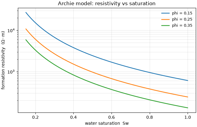
ArchieModel gives formation resistivity as a function of porosity and water saturation. Sweeping saturation at a fixed porosity shows the strong resistivity increase as pores drain.

import matplotlib.pyplot as plt
import numpy as np

from pycsamt.interp.petrophysics import (
    ArchieModel,
    HashinShtrikmanBounds,
    kozeny_carman_K,
)

# Use the resistivity vs porosity model curve (2nd figure) as the thumbnail.

archie = ArchieModel(m=1.8, n=2.0, a=1.0)
Sw = np.linspace(0.15, 1.0, 60)
rho_w = 20.0
fig, ax = plt.subplots(figsize=(6.5, 4.2), constrained_layout=True)
for phi in (0.15, 0.25, 0.35):
    rho = np.array([archie.forward(phi=phi, Sw=s, rho_w=rho_w) for s in Sw])
    ax.plot(Sw, rho, lw=1.8, label=f"phi = {phi:.2f}")
ax.set_yscale("log")
ax.set_xlabel("water saturation  Sw")
ax.set_ylabel(r"formation resistivity  ($\Omega\cdot$m)")
ax.set_title("Archie model: resistivity vs saturation")
ax.legend(frameon=False, fontsize=9)
ax.grid(alpha=0.3, which="both")

Mixing bounds and the porosity trend

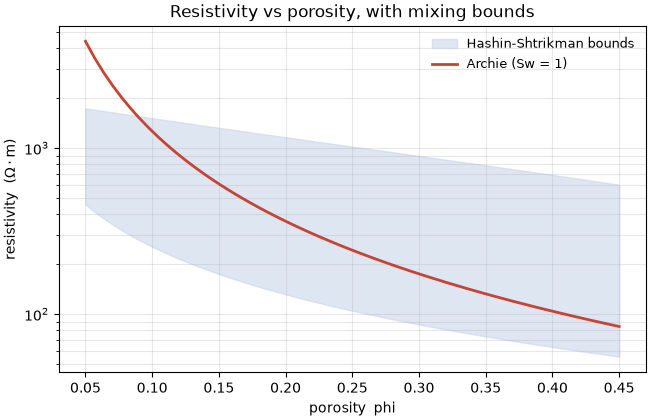
At full saturation, resistivity falls with porosity. The HashinShtrikmanBounds bracket the physically-possible range for a two-phase mix (matrix + pore fluid); the Archie curve should sit inside them.

phi = np.linspace(0.05, 0.45, 60)
rho_archie = np.array(
    [archie.forward(phi=p, Sw=1.0, rho_w=rho_w) for p in phi]
)
hs = HashinShtrikmanBounds(rho_matrix=2000.0, rho_fluid=rho_w)
lo, hi = np.array([hs.bounds(phi=p) for p in phi]).T

fig, ax = plt.subplots(figsize=(6.5, 4.2), constrained_layout=True)
ax.fill_between(
    phi, lo, hi, color="#c9d6ea", alpha=0.6, label="Hashin-Shtrikman bounds"
)
ax.plot(phi, rho_archie, color="#c44536", lw=2.0, label="Archie (Sw = 1)")
ax.set_yscale("log")
ax.set_xlabel("porosity  phi")
ax.set_ylabel(r"resistivity  ($\Omega\cdot$m)")
ax.set_title("Resistivity vs porosity, with mixing bounds")
ax.legend(frameon=False, fontsize=9)
ax.grid(alpha=0.3, which="both")

Hydraulic conductivity from porosity

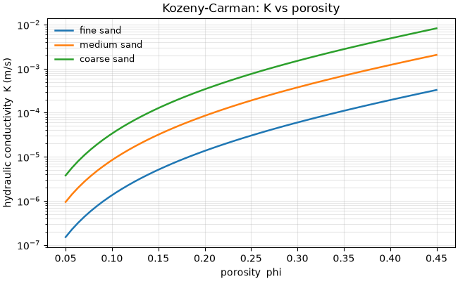
kozeny_carman_K() converts porosity (and a grain size) into hydraulic conductivity — the link from a petrophysical estimate to an aquifer property.

fig, ax = plt.subplots(figsize=(6.5, 4.0), constrained_layout=True)
for d50, lbl in [
    (2e-4, "fine sand"),
    (5e-4, "medium sand"),
    (1e-3, "coarse sand"),
]:
    K = np.array([kozeny_carman_K(p, d50_m=d50) for p in phi])
    ax.plot(phi, K, lw=1.8, label=lbl)
ax.set_yscale("log")
ax.set_xlabel("porosity  phi")
ax.set_ylabel("hydraulic conductivity  K (m/s)")
ax.set_title("Kozeny-Carman: K vs porosity")
ax.legend(frameon=False, fontsize=9)
ax.grid(alpha=0.3, which="both")

The petrophysical cross-plot

PlotPetrophysicalCrossPlot drops every cell of the real section onto the resistivity-porosity plane, coloured by saturation, with the fitted model curve — the diagnostic for checking that the rock-physics model actually matches the data.

from _interp_data import demo_model

from pycsamt.interp import EMHydroModel, PetrophysicalConfig
from pycsamt.interp.plot import PlotPetrophysicalCrossPlot

result = EMHydroModel(
    demo_model(), PetrophysicalConfig(rho_w=20.0), method_tag="AMT"
).fit()
PlotPetrophysicalCrossPlot(result).plot()

<Figure size 700x550 with 2 Axes>

Reading it. The cross-plot’s cloud should track the model curve; cells that fall far off it flag either a wrong rock-physics assumption or genuine lithological change. These same models drive the quantitative maps in Hydro-geophysics: aquifer properties and the Monte-Carlo priors in Uncertainty quantification.