Plot a 2-D inversion section

Field teams often describe their interpretation as a 2-D section even when the inversion was run on a 3-D grid. This is not a contradiction: a vertical curtain through the 3-D resistivity volume is one of the most useful ways to communicate the result along a survey line.

This example uses the compact ModEM result sample bundled in data/modem. It demonstrates three related tasks:

• load a real ModEM inversion result folder;

• use pyCSAMT’s built-in PlotSection helper to draw a section with terrain/station context;

• compare early, middle, and final iteration sections so the interpreter can see which structures are stable and which appear only late in the inversion.

The goal is not to declare a geological interpretation from one image. The goal is to teach a careful plotting workflow: check convergence, choose the section geometry, plot the model with sensible colour limits, and inspect whether the final structure is supported by earlier iterations.

1. Imports and data location

import os
import sys
from pathlib import Path

# sphinx-gallery executes examples without __file__ (the gallery
# runner sets the working directory to this example's folder).
try:
    EXAMPLE_DIR = Path(__file__).resolve().parent
except NameError:
    EXAMPLE_DIR = Path.cwd()

import matplotlib.colors as mcolors
import matplotlib.pyplot as plt
import numpy as np
import pandas as pd


def repo_root():
    root = os.environ.get("PYCSAMT_DOCS_REPO_ROOT")
    return Path(root) if root else EXAMPLE_DIR.parents[2]


ROOT = repo_root()
if str(ROOT) not in sys.path:
    sys.path.insert(0, str(ROOT))

from pycsamt.models.modem import InversionResult, PlotMisfit
from pycsamt.models.modem.plot import PlotSection

sample_dir = ROOT / "data" / "modem" / "willy_27freq_watex_line02_sample"
figure_dir = EXAMPLE_DIR / "workspaces" / "modem_result_figures"
figure_dir.mkdir(parents=True, exist_ok=True)

if not sample_dir.exists():
    raise RuntimeError(
        f"The ModEM result sample is missing. Expected folder: {sample_dir}"
    )

2. Load the ModEM result folder

InversionResult scans a ModEM run directory and collects the artefacts it can understand: log, data, covariance, and model snapshots. The bundled sample is intentionally compact; it contains three representative model snapshots rather than every iteration written by the production run.

result = InversionResult(
    sample_dir,
    load_control=False,
    load_covariance=False,
)

print(result)
print(f"Detected mode: {result.mode}")
print(f"Parsed log records: {result.n_iter}")
print(f"Final RMS: {result.final_rms:.3f}")
print(f"Available model keys: {sorted(result.models)}")

if result.mode != "3d":
    raise RuntimeError(
        "This example expects a 3-D ModEM sample so it can extract a 2-D "
        "vertical section from the volume."
    )

InversionResult(mode='3d', n_iter=74, final_rms=3.0572, models=['iter_0000', 'iter_0030', 'iter_0073'])
Detected mode: 3d
Parsed log records: 74
Final RMS: 3.057
Available model keys: ['iter_0000', 'iter_0030', 'iter_0073']

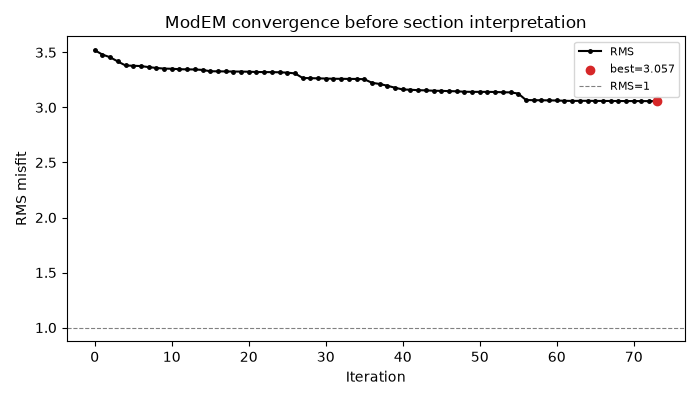
3. Check convergence before looking at the model

A beautiful section can still be a bad model if the inversion has not stabilized. Before plotting geology, quickly inspect the RMS curve. Here the final RMS remains above 1, which tells us to be cautious: use the section as a diagnostic/interpretive product, not as a final truth.

fig_misfit = PlotMisfit(result=result).plot()
fig_misfit.axes[0].set_title(
    "ModEM convergence before section interpretation"
)
misfit_file = figure_dir / "modem_sample_misfit.png"
fig_misfit.savefig(misfit_file, dpi=120)
plt.show()

4. Plot the built-in 2-D section

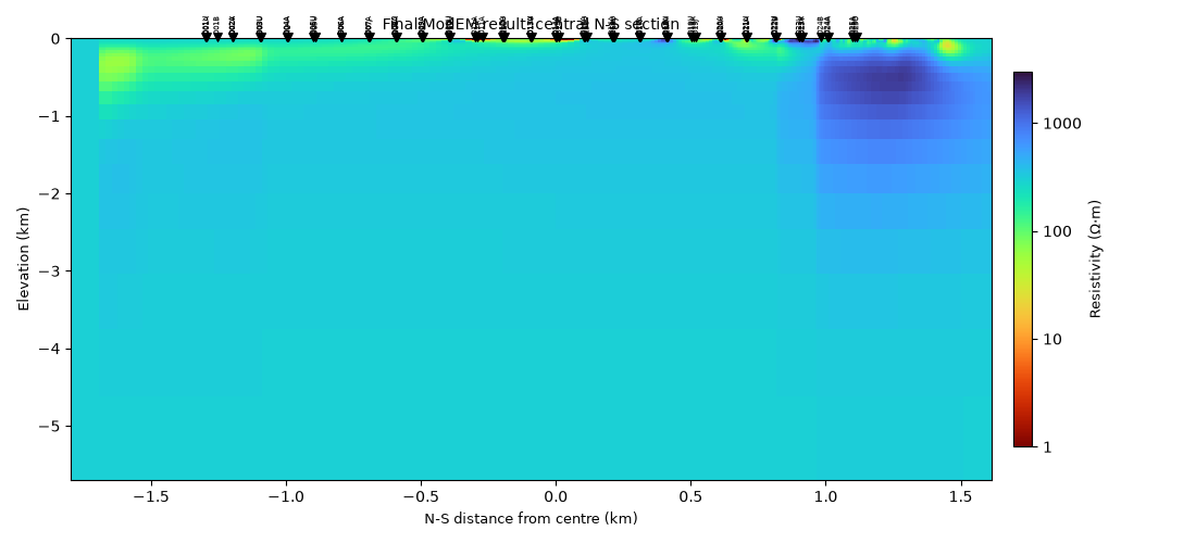
The built-in PlotSection helper extracts a North-South or East-West slice through the 3-D model. For this sample we start with a North-South section through the model centre. In a real survey you would move profile_offset until the line passes close to the stations or to the geological target.

section_offset_m = 0.0
depth_max_m = 5000.0

fig_section = PlotSection(
    result=result,
    direction="NS",
    profile_offset=section_offset_m,
    which="final",
    depth_max=depth_max_m,
    rho_min=1.0,
    rho_max=3000.0,
    cmap="turbo_r",
    show_station_names=True,
    title="Final ModEM result: central N-S section",
).plot()
section_file = figure_dir / "modem_sample_final_ns_section.png"
fig_section.savefig(section_file, dpi=120)
plt.show()

5. Build a transparent section extractor

The built-in plot is convenient, but gallery examples should also teach what is happening. The helper below extracts a section from any loaded 3-D ModEM model snapshot. The model array has shape (nz, ny, nx):

• nx is the North-South direction;

• ny is the East-West direction;

• nz is depth.

A North-South section fixes one East-West column and keeps all North-South cells. An East-West section does the opposite.

def extract_axis_section(model, direction="NS", profile_offset_m=0.0):
    direction = direction.upper()
    x_nodes = model.x_nodes
    y_nodes = model.y_nodes
    z_nodes = model.z_nodes
    x_centre = float(x_nodes[-1]) / 2.0
    y_centre = float(y_nodes[-1]) / 2.0

    if direction == "NS":
        y_target = profile_offset_m + y_centre
        y_index = int(np.argmin(np.abs(y_nodes - y_target)))
        y_index = max(0, min(y_index, model.ny - 1))
        rho = model.rho_linear[:, y_index, :]
        distance_km = (x_nodes - x_centre) / 1000.0
        label = "N-S distance from model centre (km)"
        selected_offset = float(y_nodes[y_index] - y_centre)
    elif direction == "EW":
        x_target = profile_offset_m + x_centre
        x_index = int(np.argmin(np.abs(x_nodes - x_target)))
        x_index = max(0, min(x_index, model.nx - 1))
        rho = model.rho_linear[:, :, x_index]
        distance_km = (y_nodes - y_centre) / 1000.0
        label = "E-W distance from model centre (km)"
        selected_offset = float(x_nodes[x_index] - x_centre)
    else:
        raise ValueError("direction must be 'NS' or 'EW'")

    depth_km = z_nodes / 1000.0
    return {
        "rho": rho,
        "distance_km": distance_km,
        "depth_km": depth_km,
        "distance_label": label,
        "selected_offset_m": selected_offset,
    }


def crop_section(section, max_depth_m):
    max_depth_km = max_depth_m / 1000.0
    depth_nodes = section["depth_km"]
    n_layers = int(np.searchsorted(depth_nodes, max_depth_km))
    n_layers = max(1, min(n_layers, section["rho"].shape[0]))
    cropped = dict(section)
    cropped["rho"] = section["rho"][:n_layers, :]
    cropped["depth_km"] = section["depth_km"][: n_layers + 1]
    return cropped


def thin_section(section, max_columns=90):
    """Return a lighter section for fast gallery rendering."""
    n_cols = section["rho"].shape[1]
    step = max(1, int(np.ceil(n_cols / max_columns)))
    if step == 1:
        return section
    thinned = dict(section)
    thinned["rho"] = section["rho"][:, ::step]
    thinned["distance_km"] = section["distance_km"][::step]
    if len(thinned["distance_km"]) == thinned["rho"].shape[1]:
        last_edge = section["distance_km"][-1]
        thinned["distance_km"] = np.r_[thinned["distance_km"], last_edge]
    return thinned

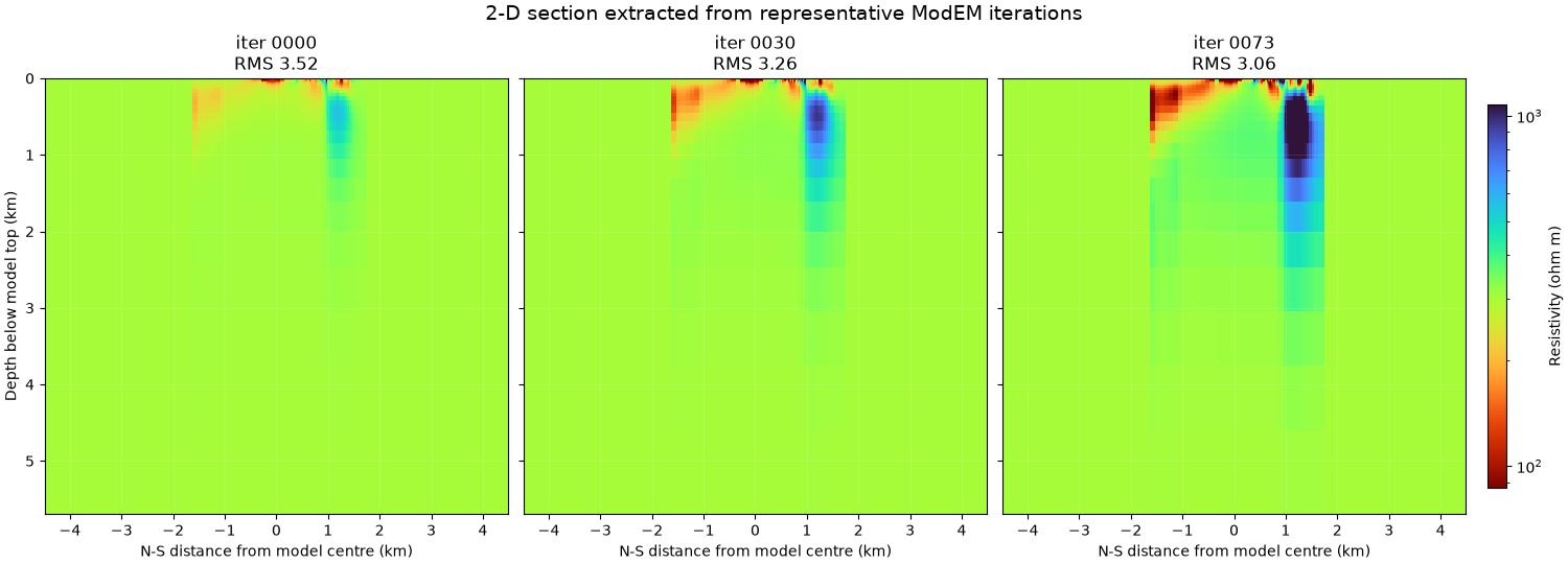
6. Compare early, middle, and final iteration sections

Stable conductors/resistors usually appear progressively. Features that appear only in the final few iterations, especially while RMS is nearly flat, should be checked against residual maps and data quality before being treated as geology.

iteration_keys = ["iter_0000", "iter_0030", "iter_0073"]
available_keys = [key for key in iteration_keys if key in result.models]
if len(available_keys) < 2:
    raise RuntimeError(
        "Need at least two model snapshots for the comparison panel. "
        f"Found: {sorted(result.models)}"
    )

sections = {
    key: thin_section(
        crop_section(
            extract_axis_section(
                result.models[key],
                direction="NS",
                profile_offset_m=section_offset_m,
            ),
            max_depth_m=depth_max_m,
        ),
    )
    for key in available_keys
}

rho_values = np.concatenate(
    [
        sec["rho"][np.isfinite(sec["rho"]) & (sec["rho"] > 0)].ravel()
        for sec in sections.values()
    ]
)
rho_min = float(np.nanpercentile(rho_values, 2))
rho_max = float(np.nanpercentile(rho_values, 98))
rho_min = max(rho_min, 1.0)
rho_max = max(rho_max, 10.0 * rho_min)

fig_compare, axes = plt.subplots(
    1,
    len(available_keys),
    figsize=(5.0 * len(available_keys), 5.4),
    sharey=True,
    constrained_layout=True,
)
if len(available_keys) == 1:
    axes = [axes]

norm = mcolors.LogNorm(vmin=rho_min, vmax=rho_max)
last_mesh = None
for ax, key in zip(axes, available_keys):
    section = sections[key]
    last_mesh = ax.pcolormesh(
        section["distance_km"],
        section["depth_km"],
        section["rho"],
        norm=norm,
        cmap="turbo_r",
        shading="flat",
    )
    iteration_number = int(key.split("_")[-1])
    rms_index = np.where(result.iteration_numbers == iteration_number)[0]
    rms_text = ""
    if rms_index.size:
        rms_text = f"\nRMS {result.rms_history[rms_index[0]]:.2f}"
    ax.set_title(f"{key.replace('_', ' ')}{rms_text}")
    ax.set_xlabel(section["distance_label"])
    ax.grid(color="white", alpha=0.15, linewidth=0.5)
    ax.invert_yaxis()

axes[0].set_ylabel("Depth below model top (km)")
colorbar = fig_compare.colorbar(last_mesh, ax=axes, shrink=0.88, pad=0.015)
colorbar.set_label("Resistivity (ohm m)")
fig_compare.suptitle(
    "2-D section extracted from representative ModEM iterations",
    fontsize=14,
)
compare_file = figure_dir / "modem_sample_iteration_section_compare.png"
fig_compare.savefig(compare_file, dpi=120)
plt.show()

7. Quantify how much the section changed

The figure is useful, but numbers help document the decision. Here we compare the logarithmic resistivity change from the starting snapshot to the final snapshot. Log-ratio is a natural scale for resistivity because a change from 10 to 100 ohm m is as important as 100 to 1000 ohm m.

first_key = available_keys[0]
final_key = available_keys[-1]
first_section = sections[first_key]["rho"]
final_section = sections[final_key]["rho"]

with np.errstate(divide="ignore", invalid="ignore"):
    log10_ratio = np.log10(final_section) - np.log10(first_section)

change_summary = pd.DataFrame(
    [
        {
            "first_snapshot": first_key,
            "final_snapshot": final_key,
            "median_abs_log10_change": float(
                np.nanmedian(np.abs(log10_ratio))
            ),
            "p90_abs_log10_change": float(
                np.nanpercentile(np.abs(log10_ratio), 90)
            ),
            "cells_changed_by_factor_10_pct": float(
                np.nanmean(np.abs(log10_ratio) >= 1.0) * 100.0
            ),
        }
    ]
)
change_file = figure_dir / "modem_sample_section_change_summary.csv"
change_summary.to_csv(change_file, index=False)
print("Section change summary:")
print(change_summary.to_string(index=False))

fig_change, ax_change = plt.subplots(
    figsize=(9.5, 5.0), constrained_layout=True
)
change_limit = max(0.5, float(np.nanpercentile(np.abs(log10_ratio), 98)))
mesh = ax_change.pcolormesh(
    sections[final_key]["distance_km"],
    sections[final_key]["depth_km"],
    log10_ratio,
    cmap="RdBu_r",
    vmin=-change_limit,
    vmax=change_limit,
    shading="flat",
)
ax_change.invert_yaxis()
ax_change.set_xlabel(sections[final_key]["distance_label"])
ax_change.set_ylabel("Depth below model top (km)")
ax_change.set_title(f"Log10 resistivity change: {first_key} to {final_key}")
cb = fig_change.colorbar(mesh, ax=ax_change, pad=0.015)
cb.set_label("log10(final / initial)")
change_plot_file = figure_dir / "modem_sample_section_log10_change.png"
fig_change.savefig(change_plot_file, dpi=120)
plt.show()

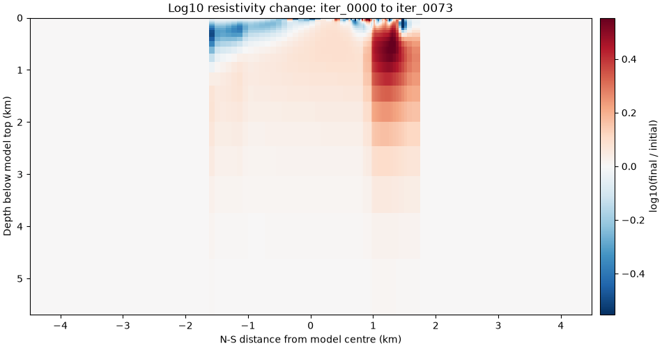
Section change summary:
first_snapshot final_snapshot  median_abs_log10_change  p90_abs_log10_change  cells_changed_by_factor_10_pct
     iter_0000      iter_0073                 0.078275              0.370318                        0.357143

8. What to inspect before interpretation

A section plot is an interpretation aid, not a certificate of truth. Before presenting the final model, check:

• whether RMS is still decreasing rapidly or has stabilized;

• whether high-amplitude structures are already visible in the mid-run model;

• whether the structures align with stations that have acceptable residuals;

• whether the colour limits hide important shallow or deep contrasts;

• whether the same feature appears on nearby parallel sections.

Files written by this example:

print(f"Misfit figure: {misfit_file}")
print(f"Built-in final section: {section_file}")
print(f"Iteration comparison: {compare_file}")
print(f"Section change plot: {change_plot_file}")
print(f"Section change table: {change_file}")

Misfit figure: /opt/build/repo/docs/examples/inversion/workspaces/modem_result_figures/modem_sample_misfit.png
Built-in final section: /opt/build/repo/docs/examples/inversion/workspaces/modem_result_figures/modem_sample_final_ns_section.png
Iteration comparison: /opt/build/repo/docs/examples/inversion/workspaces/modem_result_figures/modem_sample_iteration_section_compare.png
Section change plot: /opt/build/repo/docs/examples/inversion/workspaces/modem_result_figures/modem_sample_section_log10_change.png
Section change table: /opt/build/repo/docs/examples/inversion/workspaces/modem_result_figures/modem_sample_section_change_summary.csv