
Note
Go to the end to download the full example code.
Selecting robust site subsets#
The previous example loaded one EDI directory and built a station summary. In real projects, the next question is usually more selective:
“Which stations should I keep for this workflow?”
Selection is not the same thing as editing. The helpers in
pycsamt.site return new Sites collections and
leave the original survey untouched. This makes them safe for exploratory
notebooks, documentation examples, automated tests, and reproducible
processing recipes.
This gallery page walks through common selection patterns from simple to more robust:
remove stations with no usable impedance;
select a survey line by station-name pattern;
keep a frequency-band-compatible subset;
select deterministic station indices for examples and smoke tests;
use a small custom predicate when a project needs a rule that is not built into the public helpers.
The examples use the bundled WILLY survey, which contains several line
directories under data/AMT/WILLY_DATA.
1. Imports and bundled data#
Keep gallery imports visible and conventional. The small path bootstrap is
only here so the downloaded example can be run directly from a source tree;
during a Sphinx build, docs/source/conf.py already inserts the repo root.
import os
import re
import sys
from pathlib import Path

import matplotlib.pyplot as plt


def repo_root():
    root = os.environ.get("PYCSAMT_DOCS_REPO_ROOT")
    return Path(root) if root else Path(__file__).resolve().parents[3]


ROOT = repo_root()
if str(ROOT) not in sys.path:
    sys.path.insert(0, str(ROOT))

from pycsamt.emtools import ensure_sites
from pycsamt.site import (
    SitesReport,
    by_freq,
    by_index,
    by_names,
    by_predicate,
    drop_empty,
    keep_finite_z,
)

edi_root = ROOT / "data" / "AMT" / "WILLY_DATA"
2. Load the full WILLY survey#
Here we intentionally load the parent survey directory with
recursive=True so every line under WILLY_DATA is visible. That gives
the selectors something meaningful to do.
all_sites = ensure_sites(edi_root, recursive=True, verbose=0)
all_table = SitesReport(all_sites).to_dataframe()

print(f"Loaded WILLY survey: {len(all_sites)} station(s)")
print(
    all_table[["station", "nfreq", "freq_min", "freq_max"]]
    .head(10)
    .to_string(index=False)
)
Loaded WILLY survey: 53 station(s)
station  nfreq  freq_min  freq_max
18-001A     53     1.008   10400.0
18-002U     53     1.008   10400.0
18-003A     53     1.008   10400.0
18-004A     53     1.008   10400.0
18-005U     53     1.008   10400.0
18-006A     53     1.008   10400.0
18-007U     53     1.008   10400.0
18-008U     53     1.008   10400.0
18-009A     53     1.008   10400.0
18-010U     53     1.008   10400.0
The bundled station names encode the line number. For example, stations on
line 18 start with 18- and stations on line 22 start with 22-. A
quick grouped count makes that convention visible.
line_counts = (
    all_table["station"].str.split("-", n=1).str[0].value_counts().sort_index()
)
print("Stations by line prefix:")
print(line_counts.to_string())
Stations by line prefix:
station
18    28
22    25
3. First robustness gate: keep stations with finite impedance#
keep_finite_z is a conservative loading check. It keeps a station if it
contains at least one finite impedance value, or a finite apparent
resistivity surrogate when the raw tensor is not available.
This is not a full quality-control score. It simply answers: “does this station contain usable transfer-function data at all?”
finite_sites = keep_finite_z(all_sites)
finite_table = SitesReport(finite_sites).to_dataframe()

print(f"Before finite-Z filter: {len(all_sites)}")
print(f"After finite-Z filter:  {len(finite_sites)}")
Before finite-Z filter: 53
After finite-Z filter:  53
In many real surveys this is where broken exports, empty EDI files, or stations with only header metadata disappear. If a station is removed here, inspect the source EDI before forcing it back into later workflows.
4. Select a line by station-name pattern#
by_names accepts glob-like strings, compiled regular expressions, or
callables. Glob strings are often the most readable for survey line names.
The WILLY line-18 stations use the 18-* pattern. The result preserves
the original station order.
line18_sites = by_names(finite_sites, "18-*")
line18_table = SitesReport(line18_sites).to_dataframe()

print(f"Line 18 station count: {len(line18_sites)}")
print(
    line18_table[["station", "nfreq", "freq_min", "freq_max"]]
    .head()
    .to_string(index=False)
)
Line 18 station count: 28
station  nfreq  freq_min  freq_max
18-001A     53     1.008   10400.0
18-002U     53     1.008   10400.0
18-003A     53     1.008   10400.0
18-004A     53     1.008   10400.0
18-005U     53     1.008   10400.0
Multiple patterns are interpreted as an OR condition. This is useful when a workflow needs two lines for comparison or interpolation.
line18_or_22 = by_names(finite_sites, ["18-*", "22-*"])
line18_or_22_table = SitesReport(line18_or_22).to_dataframe()

print(f"Line 18 + line 22 station count: {len(line18_or_22)}")
print(
    line18_or_22_table["station"]
    .str.split("-", n=1)
    .str[0]
    .value_counts()
    .sort_index()
    .to_string()
)
Line 18 + line 22 station count: 53
station
18    28
22    25
5. Select stations that overlap a frequency band#
by_freq is a membership filter. It keeps a station when at least one
measured frequency lies inside the closed interval [fmin, fmax].
It does not cut rows out of each station. If you need to actually
subset the frequency axis, use the editing helpers such as
pycsamt.site.select_freq() after selecting the stations.
band_min_hz = 10.0
band_max_hz = 1_000.0

line18_band_sites = by_freq(line18_sites, band_min_hz, band_max_hz)
line18_band_table = SitesReport(line18_band_sites).to_dataframe()

print(
    f"Line 18 stations overlapping {band_min_hz:g}-{band_max_hz:g} Hz: {len(line18_band_sites)}"
)
print(
    line18_band_table[["station", "nfreq", "freq_min", "freq_max"]]
    .head()
    .to_string(index=False)
)
Line 18 stations overlapping 10-1000 Hz: 28
station  nfreq  freq_min  freq_max
18-001A     53     1.008   10400.0
18-002U     53     1.008   10400.0
18-003A     53     1.008   10400.0
18-004A     53     1.008   10400.0
18-005U     53     1.008   10400.0
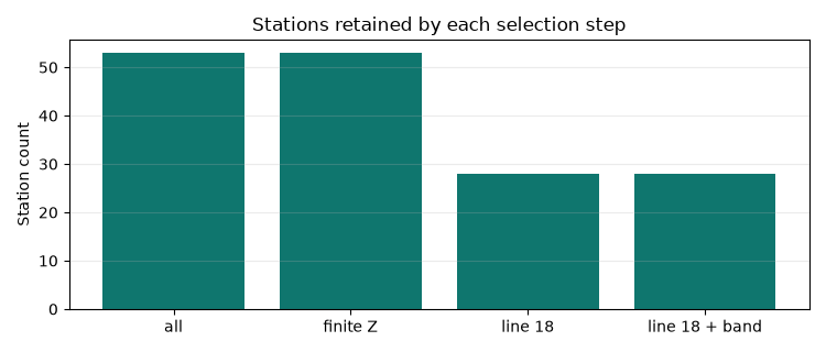
For a quick sanity check, compare how many stations remain after each step.
selection_counts = {
    "all": len(all_sites),
    "finite Z": len(finite_sites),
    "line 18": len(line18_sites),
    "line 18 + band": len(line18_band_sites),
}

print("Selection counts:")
for label, count in selection_counts.items():
    print(f"{label:14s}: {count:3d}")
Selection counts:
all           :  53
finite Z      :  53
line 18       :  28
line 18 + band:  28
A small bar plot makes that reduction easy to read in the rendered gallery.
fig, ax = plt.subplots(figsize=(7.5, 3.2))
ax.bar(selection_counts.keys(), selection_counts.values(), color="#0f766e")
ax.set_title("Stations retained by each selection step")
ax.set_ylabel("Station count")
ax.grid(axis="y", alpha=0.25)
fig.tight_layout()
6. Deterministic subsets for examples, tests, and demos#
by_index keeps stations by zero-based position. This is especially
useful when an example should stay small but still use real survey objects.
Negative indices work like normal Python indexing.
demo_sites = by_index(line18_band_sites, [0, 1, 2, -1])
demo_table = SitesReport(demo_sites).to_dataframe()

print("Small deterministic subset:")
print(
    demo_table[["station", "nfreq", "freq_min", "freq_max"]].to_string(
        index=False
    )
)
Small deterministic subset:
station  nfreq  freq_min  freq_max
18-001A     53     1.008   10400.0
18-002U     53     1.008   10400.0
18-003A     53     1.008   10400.0
18-025A     53     1.008   10400.0
Use index-based selection carefully in production pipelines. It is best for examples and smoke tests. For project recipes, name-based selection is usually clearer because it survives station-order changes.
7. Custom selection with a predicate#
When a project rule is not covered by a built-in helper, by_predicate
accepts a function that returns True for stations to keep.
The predicate receives each underlying EDI-like station object. Different
datasets expose metadata through slightly different attributes, so robust
predicates should use getattr and handle missing values gracefully.
def has_station_name_with_even_suffix(edi):
    """Keep stations whose final station-name number is even."""

    header = getattr(edi, "Head", None)
    name = getattr(header, "dataid", None) or getattr(edi, "station", "")
    match = re.search(r"(\d+)[A-Za-z]*$", str(name))
    if match is None:
        return False
    return int(match.group(1)) % 2 == 0


even_suffix_sites = by_predicate(
    line18_band_sites, has_station_name_with_even_suffix
)
even_suffix_table = SitesReport(even_suffix_sites).to_dataframe()

print(f"Line 18 stations with even numeric suffix: {len(even_suffix_sites)}")
print(even_suffix_table[["station", "nfreq"]].head(10).to_string(index=False))
Line 18 stations with even numeric suffix: 13
station  nfreq
18-002U     53
18-004A     53
18-006A     53
18-008U     53
18-010U     53
18-012A     53
18-014A     53
18-016A     53
18-018A     53
18-020A     53
8. Drop structurally empty stations when chaining selections#
drop_empty is a coarse structural check. It removes stations with no
frequency vector, no impedance container, or no usable arrays. It can be a
useful final guard in defensive scripts.
clean_demo_sites = drop_empty(demo_sites)
clean_demo_table = SitesReport(clean_demo_sites).to_dataframe()

print(f"Demo subset before drop_empty: {len(demo_sites)}")
print(f"Demo subset after drop_empty:  {len(clean_demo_sites)}")
print(
    clean_demo_table[
        ["station", "has_Zxy", "has_Zyx", "has_tipper"]
    ].to_string(index=False)
)
Demo subset before drop_empty: 4
Demo subset after drop_empty:  4
station  has_Zxy  has_Zyx  has_tipper
18-001A     True     True       False
18-002U     True     True       False
18-003A     True     True       False
18-025A     True     True       False
9. Recommended selection pattern#
For a typical scripted workflow, prefer a short, readable chain:
sites = ensure_sites(edi_dir, recursive=True, verbose=0)
sites = keep_finite_z(sites)
sites = by_names(sites, "18-*")
sites = by_freq(sites, 10.0, 1_000.0)
sites = drop_empty(sites)
The original all_sites object remains available for comparison, and each
step can be reported independently. That makes selection choices explicit
for the next developer who reads the notebook, gallery page, or test.
Total running time of the script: (0 minutes 0.372 seconds)