Uncertainty and calibration

A point prediction is not enough — an AI inverter must say how sure it is. This example covers the two questions that matter in practice:

1. How uncertain is each prediction? — via a deep ensemble (EnsembleInverter), whose spread across members estimates epistemic uncertainty.

2. Are those uncertainties honest? — via conformal prediction (ConformalPredictor), which turns raw spreads into intervals with a guaranteed coverage rate, and lets us check that guarantee empirically.

Dataset and ensemble

An EnsembleInverter trains several copies of a base inverter from different random seeds. At prediction time the member mean is the estimate and the member spread is the uncertainty.

# Use the depth-profile uncertainty band (1st figure) as the thumbnail.
import os

import numpy as np

from pycsamt.ai.inversion import EnsembleInverter
from pycsamt.ai.inversion.inv1d import EMInverter1D
from pycsamt.forward.batch import generate_dataset

# Lighter training while building the docs (PYCSAMT_DOCS_BUILD is set by Sphinx);
# full strength when the example is run directly.
_DOCS = bool(os.environ.get("PYCSAMT_DOCS_BUILD"))

N_LAYERS = 4
FREQS = np.logspace(-1, 3, 24)
ds = generate_dataset(
    solver="mt1d",
    n_samples=256 if _DOCS else 1200,
    freqs=FREQS,
    n_layers=N_LAYERS,
    noise_level=0.05,
    seed=2,
    verbose=False,
)
train, cal, test = ds.split()  # reuse the "val" split for calibration

base = EMInverter1D(arch="cnn1d", n_layers=N_LAYERS, solver="mt1d")
ens = EnsembleInverter(base_estimator=base, n_estimators=2 if _DOCS else 4)
ens.fit(train, epochs=5 if _DOCS else 20, verbose=False)

mean, std = ens.predict_with_uncertainty(test.X)
print("ensemble mean/std shapes:", mean.shape, std.shape)

ensemble mean/std shapes: (25, 7) (25, 7)

A prediction interval as a depth profile

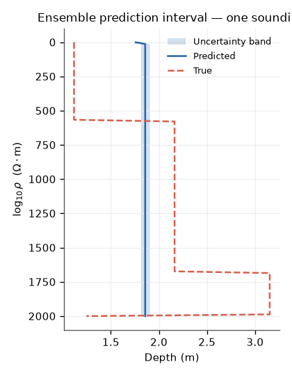
The ensemble returns a mean and standard deviation for every model parameter. We expand one test sounding’s resistivity layers (mean ± 1 std) onto a depth axis and draw it with plot_uncertainty_bands(). The shaded band is the ensemble’s confidence; the dashed line is ground truth.

from pycsamt.ai.plot import plot_uncertainty_bands


def to_depth_profile(row, srow=None, depth_max=2000.0, n=160):
    """Expand a [log_rho(L), thickness_m(L-1)] vector onto a depth axis."""
    logrho = row[:N_LAYERS]
    thick = np.maximum(row[N_LAYERS:], 1.0)  # thickness is in metres
    depths = np.linspace(0, depth_max, n)
    edges = np.concatenate([[0.0], np.cumsum(thick), [np.inf]])
    prof = np.empty_like(depths)
    band = np.zeros_like(depths)
    for i in range(N_LAYERS):
        m = (depths >= edges[i]) & (depths < edges[i + 1])
        prof[m] = logrho[i]
        if srow is not None:
            band[m] = srow[i]
    return depths, prof, band


i = 0
depths, mprof, mband = to_depth_profile(mean[i], std[i])
_, tprof, _ = to_depth_profile(test.y[i])
fig = plot_uncertainty_bands(
    depths,
    mprof,
    mprof + mband,
    mprof - mband,
    y_true=tprof,
    xlabel="Depth (m)",
    ylabel=r"$\log_{10}\rho$  ($\Omega\cdot$m)",
    title="Ensemble prediction interval — one sounding",
)

Calibrate with conformal prediction

Raw ensemble spreads are often mis-scaled. ConformalPredictor uses a held-out calibration set to rescale them so that, e.g., a nominal 90% interval really contains the truth ~90% of the time — a distribution- free guarantee.

from pycsamt.ai.inversion import ConformalPredictor

cp = ConformalPredictor(ens).calibrate(cal.X, cal.y, alpha=0.10)
center, lo, hi = cp.predict_intervals(test.X)
inside = np.mean((test.y >= lo) & (test.y <= hi))
print(f"empirical coverage of the nominal 90% interval: {inside:.2%}")

empirical coverage of the nominal 90% interval: 100.00%

Is the uncertainty honest? A reliability curve

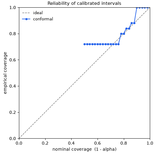
coverage_diagnostics() returns empirical coverage across a sweep of nominal levels. A well-calibrated predictor lies on the diagonal — every point above it means “conservative” (intervals a bit wide), below means “overconfident”.

import matplotlib.pyplot as plt

diag = cp.coverage_diagnostics(test.X, test.y)
alphas = np.array(sorted(diag))
nominal = 1.0 - alphas
empirical = np.array([diag[a] for a in alphas])

fig, ax = plt.subplots(figsize=(5.2, 5.0), constrained_layout=True)
ax.plot([0, 1], [0, 1], ls="--", color="0.5", lw=1.2, label="ideal")
ax.plot(nominal, empirical, "o-", color="#2563eb", ms=4, label="conformal")
ax.set_xlabel("nominal coverage  (1 - alpha)")
ax.set_ylabel("empirical coverage")
ax.set_title("Reliability of calibrated intervals", fontsize=11)
ax.set_xlim(0, 1)
ax.set_ylim(0, 1)
ax.set_aspect("equal")
ax.legend(frameon=False, fontsize=9)

<matplotlib.legend.Legend object at 0x7f2aa82a8140>

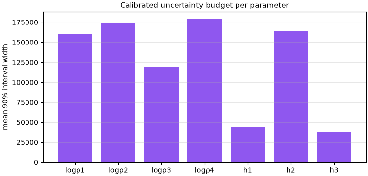
Interval width per parameter

The calibrated interval width is the practical uncertainty budget. Wider bars mean the network is less certain about that parameter — typically the deeper layers and their thicknesses.

widths = (hi - lo).mean(axis=0)
labels = [f"logρ{j + 1}" for j in range(N_LAYERS)] + [
    f"h{j + 1}" for j in range(N_LAYERS - 1)
]
fig, ax = plt.subplots(figsize=(7.5, 3.6), constrained_layout=True)
ax.bar(labels, widths, color="#7c3aed", alpha=0.85)
ax.set_ylabel("mean 90% interval width")
ax.set_title("Calibrated uncertainty budget per parameter", fontsize=11)
ax.grid(axis="y", alpha=0.3)

Takeaway. Ensembles give a cheap uncertainty estimate; conformal calibration makes it trustworthy. Report calibrated intervals — not bare point predictions — whenever an AI inversion feeds a downstream decision. The same predict_with_uncertainty API returns Monte-Carlo-dropout uncertainty for the 2-D and 3-D inverters in the next examples.