The resistivity model

Everything in pycsamt.interp starts from a ResistivityModel — a 2-D section of \(\log_{10}\rho\) on a (depth, distance) grid, plus station positions and metadata. It usually comes from an inversion (ResistivityModel.from_occam2d), but you can build one directly from arrays, which is what this whole gallery does so every deliverable traces back to a known model.

This first example builds the shared synthetic section and reads it as 1-D resistivity-depth profiles.

Build a model from arrays

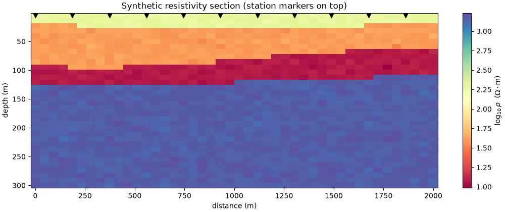
ResistivityModel.from_array takes a (n_z, n_x) array of \(\log_{10}\rho\) with cell-centre depth and distance axes. Here the section is a classic hydrogeological sequence: a resistive dry overburden, a conductive sand aquifer, a very conductive clay aquitard, and a resistive basement.

import matplotlib.pyplot as plt
import numpy as np
from _interp_data import demo_model

# Use the resistivity section (2nd figure) as the card thumbnail.

rm = demo_model()
print(rm)
print(
    "grid (n_z, n_x):",
    rm.rho_2d.shape,
    f" depth 0-{rm.z_centers.max():.0f} m,  distance 0-{rm.x_centers.max():.0f} m",
)

ResistivityModel(x_centers=array([   0.        ,   46.51162791,   93.02325581,  139.53488372,
        186.04651163,  232.55813953,  279.06976744,  325.58139535,
        372.09302326,  418.60465116,  465.11627907,  511.62790698,
        558.13953488,  604.65116279,  651.1627907 ,  697.6744186 ,
        744.18604651,  790.69767442,  837.20930233,  883.72093023,
        930.23255814,  976.74418605, 1023.25581395, 1069.76744186,
       1116.27906977, 1162.79069767, 1209.30232558, 1255.81395349,
       1302.3255814 , 1348.8372093 , 1395.34883721, 1441.86046512,
       1488.37209302, 1534.88372093, 1581.39534884, 1627.90697674,
       1674.41860465, 1720.93023256, 1767.44186047, 1813.95348837,
       1860.46511628, 1906.97674419, 1953.48837209, 2000.        ]), z_centers=array([  5.        ,  13.93939394,  22.87878788,  31.81818182,
        40.75757576,  49.6969697 ,  58.63636364,  67.57575758,
        76.51515152,  85.45454545,  94.39393939, 103.33333333,
       112.27272727, 121.21212121, 130.15151515, 139.09090909,
       148.03030303, 156.96969697, 165.90909091, 174.84848485,
       183.78787879, 192.72727273, 201.66666667, 210.60606061,
       219.54545455, 228.48484848, 237.42424242, 246.36363636,
       255.3030303 , 264.24242424, 273.18181818, 282.12121212,
       291.06060606, 300.        ]), rho_2d=array([[2.30375165, 2.29815186, 2.31471859, ..., 2.33271963, 2.32931397,
        2.31767295],
       [2.30673494, 2.29415918, 2.33158966, ..., 2.31450789, 2.31346997,
        2.32826865],
       [1.58535681, 1.63727168, 1.59577418, ..., 1.5791018 , 1.57879958,
        1.60784983],
       ...,
       [3.17388868, 3.17022536, 3.18401731, ..., 3.20653867, 3.19037284,
        3.18860291],
       [3.19206417, 3.15233639, 3.17534221, ..., 3.120498  , 3.19527903,
        3.15272897],
       [3.19963319, 3.18334056, 3.18957228, ..., 3.15714982, 3.20185913,
        3.14551675]], shape=(34, 44)), station_x=array([   0.        ,  186.04651163,  372.09302326,  558.13953488,
        744.18604651,  930.23255814, 1116.27906977, 1302.3255814 ,
       1488.37209302, 1674.41860465, 1860.46511628]), station_names=['S00', 'S01', 'S02', 'S03', 'S04', 'S05', 'S06', 'S07', 'S08', 'S09', 'S10'], method='synthetic', rms=nan)
grid (n_z, n_x): (34, 44)  depth 0-300 m,  distance 0-2000 m

The section itself

A quick look at the model with an EM-style colour scale: cool colours are conductive (water, clay), warm colours resistive (dry ground, basement).

fig, ax = plt.subplots(figsize=(10, 4.2), constrained_layout=True)
im = ax.pcolormesh(
    rm.x_centers, rm.z_centers, rm.rho_2d, cmap="Spectral", shading="auto"
)
ax.plot(
    rm.station_x,
    np.full_like(rm.station_x, rm.z_centers.min()),
    "kv",
    ms=6,
    clip_on=False,
)
ax.invert_yaxis()
ax.set_xlabel("distance (m)")
ax.set_ylabel("depth (m)")
ax.set_title("Synthetic resistivity section (station markers on top)")
fig.colorbar(im, ax=ax, label=r"$\log_{10}\rho$  ($\Omega\cdot$m)")

<matplotlib.colorbar.Colorbar object at 0x7f2aa34a2090>

1-D resistivity-depth profiles

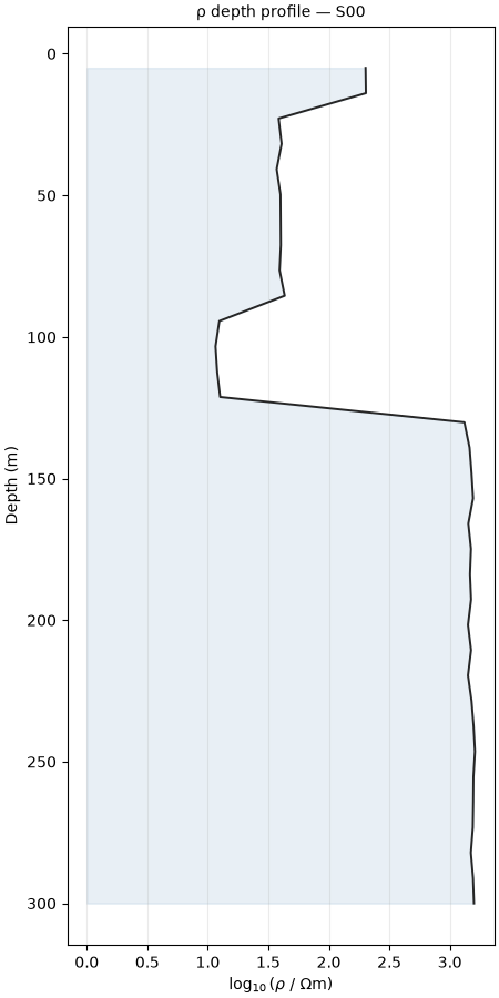
PlotResistivityDepthProfile extracts the sounding beneath a station and plots resistivity against depth — the most direct way to pick layer boundaries. Passing a ResistivityModel shows the raw log; later examples pass an EMHydroResult to add zone shading.

from pycsamt.interp.plot import PlotResistivityDepthProfile

PlotResistivityDepthProfile(rm).plot()

<Figure size 450x900 with 1 Axes>

Reading it. The profile drops sharply into the aquifer (~40 Ohm-m near 20 m), bottoms out in the clay (~12 Ohm-m), then rises steeply into the resistive basement (>1000 Ohm-m). Those four segments are exactly what the lithology and hydro examples turn into named units and aquifer zones.