2-D MT forward models and pseudo-sections

Real structure is rarely 1-D. Grid2D discretises a resistivity cross-section and MT2DForward runs a finite-difference MT solver over it, returning TE- and TM-mode apparent resistivity and phase at every station and frequency. This example builds two end-member targets — a conductive fault zone and a resistive intrusion — and works through the full set of 2-D views: the model itself, TE/TM pseudo-sections, lateral response profiles, and a combined “validate” panel.

Two 2-D targets

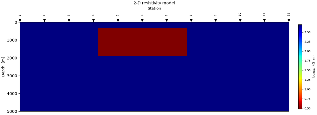
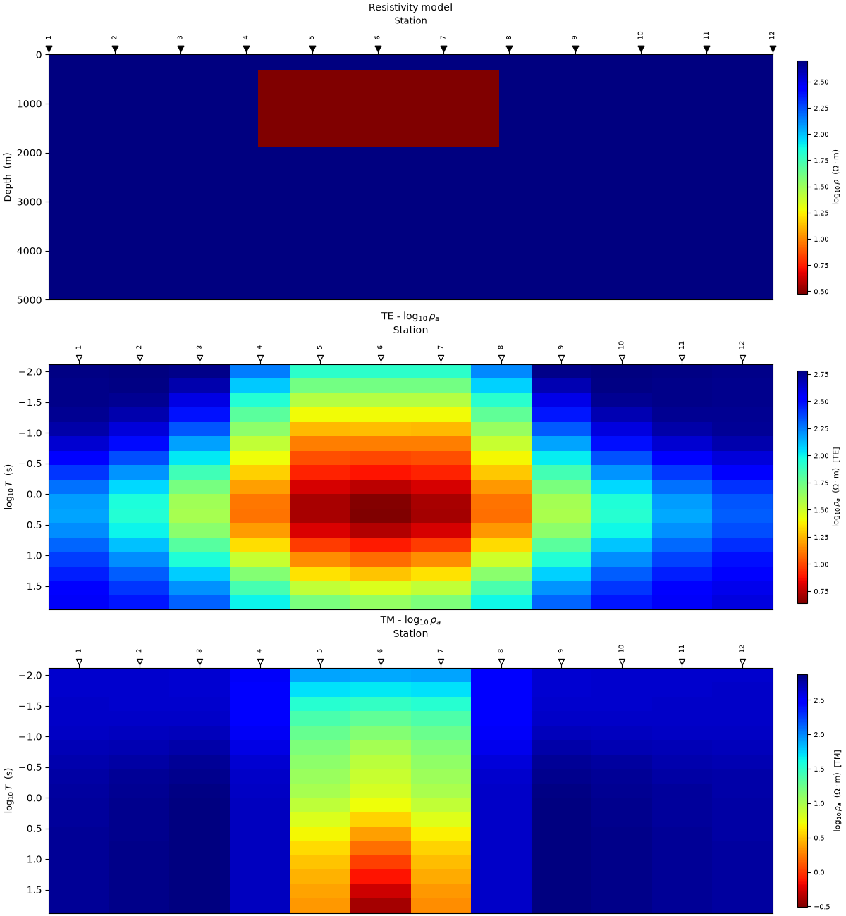
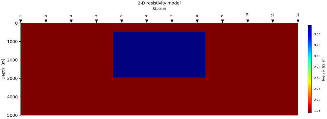
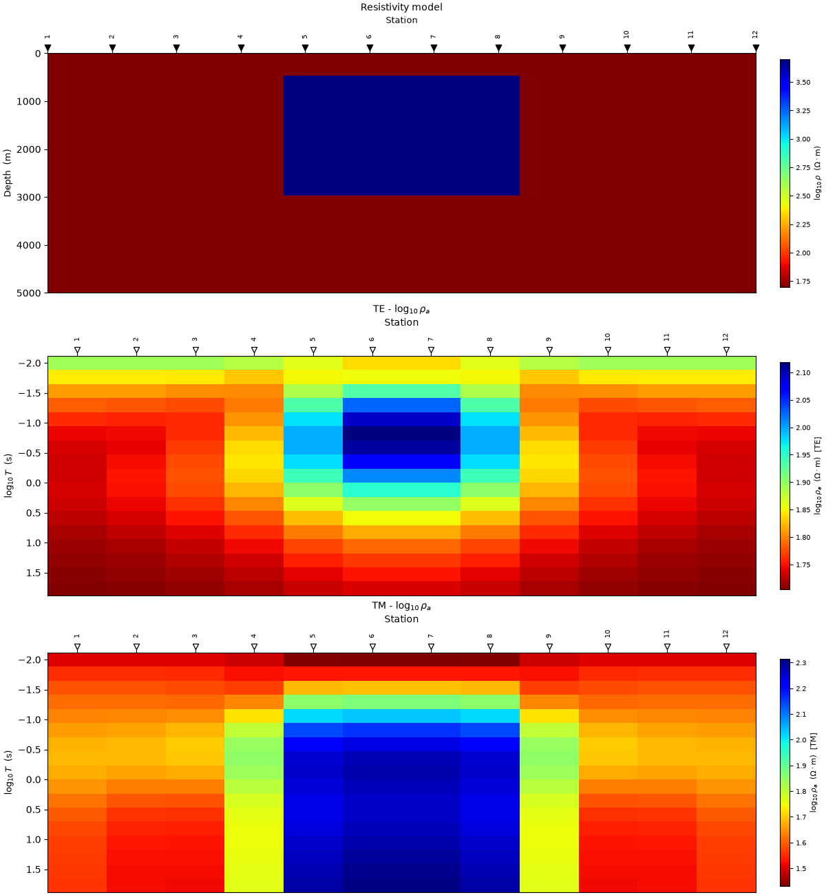
Grid2D.with_anomaly embeds a rectangular anomaly in a uniform background. Model A is a 3 Ohm-m conductor in a 500 Ohm-m host (a fault zone / graphite schist); Model B is a 5000 Ohm-m block in a 50 Ohm-m host (a salt dome / igneous intrusion). Both use 12 stations and a padded 45x32 mesh.

import matplotlib.pyplot as plt
import numpy as np

from pycsamt.forward import (
    Grid2D,
    MT2DForward,
    plot_model_2d,
    plot_pseudosection_2d,
    plot_response_profiles,
)

# Use the fault-zone validate panel (9th figure) as the section thumbnail.

FREQS_2D = np.logspace(-2, 2, 18)  # 0.01 - 100 Hz

GRID_FAULT = Grid2D.with_anomaly(
    bg_rho=500.0,
    anomaly_rho=3.0,
    anomaly_bounds=(2_500.0, 5_500.0, 300.0, 1_800.0),
    nx=45,
    nz=32,
    x_max=9_000.0,
    z_max=5_000.0,
    n_stations=12,
    n_pad=8,
    name="fault-zone conductor",
)
GRID_SALT = Grid2D.with_anomaly(
    bg_rho=50.0,
    anomaly_rho=5_000.0,
    anomaly_bounds=(3_000.0, 6_000.0, 500.0, 3_000.0),
    nx=45,
    nz=32,
    x_max=9_000.0,
    z_max=5_000.0,
    n_stations=12,
    n_pad=8,
    name="resistive intrusion",
)

RESP_FAULT = MT2DForward(FREQS_2D, GRID_FAULT, verbose=False).run()
RESP_SALT = MT2DForward(FREQS_2D, GRID_SALT, verbose=False).run()

1. The resistivity models

plot_model_2d() renders the mesh as a log-resistivity image with station markers along the top.

ax = plot_model_2d(GRID_FAULT, figsize=(11, 4))

The resistive intrusion is the polarity-reversed case — a high-resistivity block in a conductive host:

ax = plot_model_2d(GRID_SALT, figsize=(11, 4))

2. TE and TM pseudo-sections

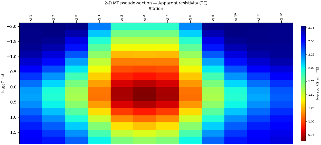
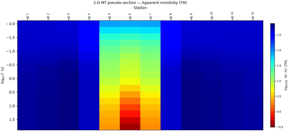
plot_pseudosection_2d() images apparent resistivity (or phase) across station-vs-period. The two polarisation modes see the fault differently: TE (electric field along strike) smears the conductor laterally, while TM (across strike) keeps it sharp — the classic reason both modes are modelled and inverted together.

ax = plot_pseudosection_2d(
    RESP_FAULT, mode="te", quantity="rho_a", figsize=(11, 5)
)

ax = plot_pseudosection_2d(
    RESP_FAULT, mode="tm", quantity="rho_a", figsize=(11, 5)
)

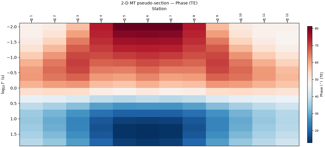
The same TE data as phase rather than apparent resistivity — phase leads the resistivity contrast and often flags the anomaly edges more crisply:

ax = plot_pseudosection_2d(
    RESP_FAULT, mode="te", quantity="phase", figsize=(11, 5)
)

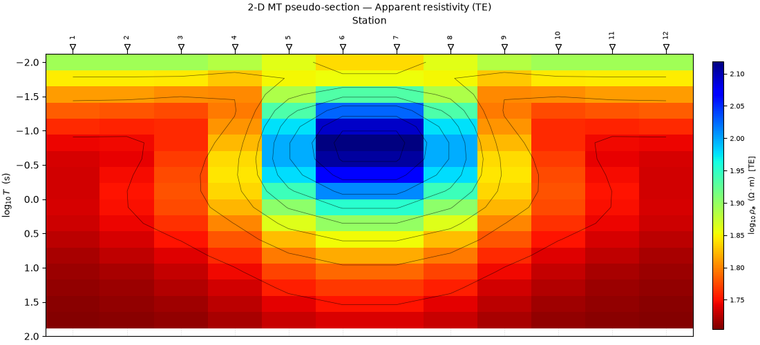
For the resistive intrusion, adding contour lines (n_contours) makes the resistive core and its overprint on the section stand out:

ax = plot_pseudosection_2d(
    RESP_SALT, mode="te", quantity="rho_a", n_contours=8, figsize=(11, 5)
)

3. Lateral response profiles

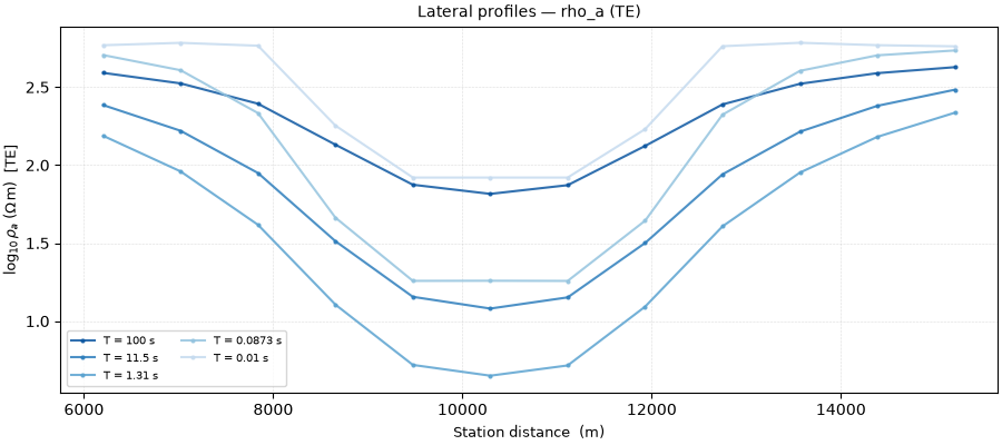
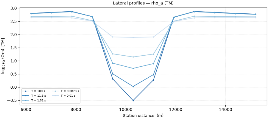
plot_response_profiles() slices the pseudo-section the other way: apparent resistivity along the profile at a few selected periods, so you can read the anomaly’s lateral extent directly. TE and TM again disagree over the conductor.

ax = plot_response_profiles(
    RESP_FAULT, mode="te", quantity="rho_a", n_freqs_shown=5, figsize=(9, 4)
)

ax = plot_response_profiles(
    RESP_FAULT, mode="tm", quantity="rho_a", n_freqs_shown=5, figsize=(9, 4)
)

4. The combined validate panel

The plotting helpers accept an ax= argument, so the model and both modes stack into one figure — a compact, publication-ready summary of a 2-D forward run. This is the figure to save when documenting a synthetic test.

fig, axs = plt.subplots(3, 1, figsize=(12, 13), constrained_layout=True)
plot_model_2d(
    GRID_FAULT, ax=axs[0], show_stations=True, title="Resistivity model"
)
plot_pseudosection_2d(
    RESP_FAULT,
    ax=axs[1],
    mode="te",
    quantity="rho_a",
    show_stations=True,
    title=r"TE - $\log_{10}\rho_a$",
)
plot_pseudosection_2d(
    RESP_FAULT,
    ax=axs[2],
    mode="tm",
    quantity="rho_a",
    show_stations=True,
    title=r"TM - $\log_{10}\rho_a$",
)
fig.suptitle(
    "2-D forward validate view - fault-zone conductor", y=1.01, fontsize=11
)

Text(0.5, 1.01, '2-D forward validate view - fault-zone conductor')

The same three-row summary for the resistive intrusion:

fig, axs = plt.subplots(3, 1, figsize=(12, 13), constrained_layout=True)
plot_model_2d(
    GRID_SALT, ax=axs[0], show_stations=True, title="Resistivity model"
)
plot_pseudosection_2d(
    RESP_SALT,
    ax=axs[1],
    mode="te",
    quantity="rho_a",
    show_stations=True,
    title=r"TE - $\log_{10}\rho_a$",
)
plot_pseudosection_2d(
    RESP_SALT,
    ax=axs[2],
    mode="tm",
    quantity="rho_a",
    show_stations=True,
    title=r"TM - $\log_{10}\rho_a$",
)
fig.suptitle(
    "2-D forward validate view - resistive intrusion", y=1.01, fontsize=11
)

Text(0.5, 1.01, '2-D forward validate view - resistive intrusion')