Build a starting model and depth grid

An inversion workspace needs more than data files. It also needs a defensible model grid: horizontal cells tied to station spacing, vertical layers tied to penetration depth, padding outside the survey, and a starting resistivity that does not secretly impose an interpretation.

This example builds a solver-neutral starting model from corrected EDIs. It does not create a ModEM or Occam control file yet; instead it writes clear grid/model artefacts that later examples can translate to a specific backend.

The design uses four pieces of evidence:

• station chainage and spacing;

• station elevation/topography;

• measured frequency range;

• Bostick depth estimates from the observed impedance.

1. Imports and paths

import csv
import json
import os
import sys
from pathlib import Path

# sphinx-gallery executes examples without __file__ (the gallery
# runner sets the working directory to this example's folder).
try:
    EXAMPLE_DIR = Path(__file__).resolve().parent
except NameError:
    EXAMPLE_DIR = Path.cwd()

import matplotlib.pyplot as plt
import numpy as np


def repo_root():
    root = os.environ.get("PYCSAMT_DOCS_REPO_ROOT")
    return Path(root) if root else EXAMPLE_DIR.parents[2]


ROOT = repo_root()
if str(ROOT) not in sys.path:
    sys.path.insert(0, str(ROOT))

from pycsamt.emtools import bostick_depth, depth_coverage_table, ensure_sites
from pycsamt.topo import (
    extract_chainage,
    extract_elevation,
    extract_station_names,
    interp_elev,
)

edi_dir = ROOT / "data" / "AMT" / "WILLY_DATA" / "L18PLT"
workspace = EXAMPLE_DIR / "workspaces" / "l18_prepared_workspace"
model_dir = workspace / "03_model_placeholder"
figure_dir = workspace / "05_figures"
table_dir = workspace / "02_tables"

for path in (model_dir, figure_dir, table_dir):
    path.mkdir(parents=True, exist_ok=True)

sites = ensure_sites(edi_dir, recursive=False, verbose=0)

2. Survey geometry controls horizontal cells

The inner model should resolve station-to-station changes without pretending to know more than the data support. A practical first pass is:

• use cell width near half the median station spacing;

• add padding on both sides of the line;

• grow padding geometrically away from the data.

station_names = extract_station_names(sites)
chain_km = extract_chainage(sites)
elev_m = extract_elevation(sites)

spacing_m = np.diff(chain_km) * 1000.0
median_spacing_m = float(np.nanmedian(spacing_m))
inner_dx_m = max(25.0, 0.5 * median_spacing_m)
line_length_m = float((chain_km[-1] - chain_km[0]) * 1000.0)

padding_cells = 8
padding_growth = 1.35
pad_widths_m = inner_dx_m * padding_growth ** np.arange(padding_cells)
left_padding_m = pad_widths_m[::-1]
right_padding_m = pad_widths_m

inner_edges_m = np.arange(0.0, line_length_m + inner_dx_m, inner_dx_m)
if inner_edges_m[-1] < line_length_m:
    inner_edges_m = np.r_[inner_edges_m, line_length_m]

x_edges_m = np.r_[
    -np.cumsum(left_padding_m),
    inner_edges_m,
    line_length_m + np.cumsum(right_padding_m),
]
x_edges_m = np.unique(np.sort(x_edges_m))
x_centres_m = 0.5 * (x_edges_m[:-1] + x_edges_m[1:])

print(f"Stations: {len(station_names)}")
print(f"Line length: {line_length_m:.1f} m")
print(f"Median station spacing: {median_spacing_m:.1f} m")
print(f"Inner cell width: {inner_dx_m:.1f} m")
print(f"Horizontal cells including padding: {len(x_centres_m)}")

Stations: 28
Line length: 19661.6 m
Median station spacing: 701.2 m
Inner cell width: 350.6 m
Horizontal cells including padding: 73

3. Frequency content controls target depth

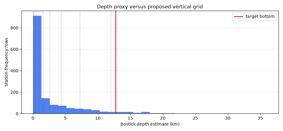
Bostick depth is not an inversion result. It is a planning proxy: a way to ask whether the chosen depth grid is broadly compatible with the data’s frequency content and apparent resistivity.

depth_table = bostick_depth(sites, recursive=False)
coverage = depth_coverage_table(sites, recursive=False)

rho_background = float(np.nanmedian(depth_table["rho_a_ohmm"]))
d10, d50, d90 = np.nanpercentile(depth_table["depth_m"], [10, 50, 90])
target_depth_m = float(max(1.5 * d90, 3.0 * d50))
target_depth_m = min(max(target_depth_m, 500.0), 15000.0)

print(f"Median apparent resistivity: {rho_background:.1f} ohm.m")
print(
    f"Bostick depth percentiles: p10={d10:.0f} m, p50={d50:.0f} m, p90={d90:.0f} m"
)
print(f"Chosen model target depth: {target_depth_m:.0f} m")

Median apparent resistivity: 317.9 ohm.m
Bostick depth percentiles: p10=52 m, p50=554 m, p90=8497 m
Chosen model target depth: 12745 m

4. Build vertical layers

A robust first-pass vertical grid has fine shallow layers and gradually thickening deeper layers. The exact solver may later require different conventions, but the design principle remains:

• first cell thickness should be small relative to station spacing;

• layers should grow smoothly;

• the bottom should be deeper than the data’s expected penetration.

first_dz_m = max(5.0, min(25.0, inner_dx_m / 4.0))
growth_z = 1.18

z_edges_m = [0.0]
dz = first_dz_m
while z_edges_m[-1] < target_depth_m:
    z_edges_m.append(z_edges_m[-1] + dz)
    dz *= growth_z
z_edges_m = np.asarray(z_edges_m, dtype=float)
z_centres_m = 0.5 * (z_edges_m[:-1] + z_edges_m[1:])

print(f"First vertical cell: {first_dz_m:.1f} m")
print(f"Vertical layers: {len(z_centres_m)}")
print(f"Bottom depth: {z_edges_m[-1]:.0f} m")

First vertical cell: 25.0 m
Vertical layers: 28
Bottom depth: 14162 m

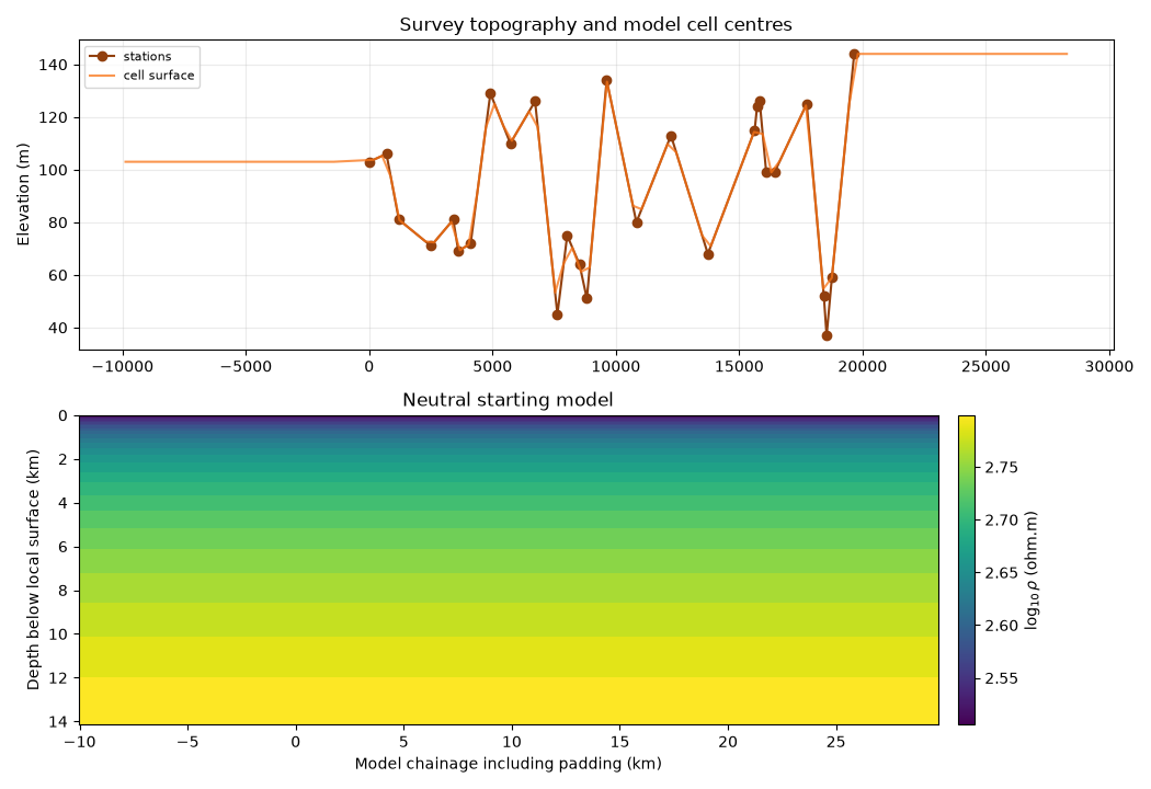
5. Build a neutral starting resistivity model

A starting model should be boring unless you have strong independent geology. Here we use a homogeneous background equal to the survey median apparent resistivity, then add a gentle depth trend. The trend prevents an unrealistically sharp uniform model without imposing a target anomaly.

X, Z = np.meshgrid(x_centres_m, z_centres_m)
log10_background = np.log10(max(rho_background, 1.0))
depth_trend = 0.18 * np.log10(1.0 + Z / 300.0)
log10_model = log10_background + depth_trend
rho_model = 10.0**log10_model

print(
    f"Starting model range: {rho_model.min():.1f}-{rho_model.max():.1f} ohm.m"
)

Starting model range: 320.2-629.6 ohm.m

6. Add topography context

The starting model is stored as depth below local surface. For plotting and later mesh work, we also compute a terrain-following elevation grid.

surface_km_at_cells = interp_elev(
    chain_km, elev_m / 1000.0, x_centres_m / 1000.0
)
surface_m_at_cells = surface_km_at_cells * 1000.0
elevation_centres_m = (
    surface_m_at_cells[np.newaxis, :] - z_centres_m[:, np.newaxis]
)

fig, axs = plt.subplots(2, 1, figsize=(10.5, 7.2), sharex=False)

axs[0].plot(
    chain_km * 1000.0, elev_m, "o-", color="#92400e", label="stations"
)
axs[0].plot(
    x_centres_m,
    surface_m_at_cells,
    "-",
    color="#f97316",
    alpha=0.75,
    label="cell surface",
)
axs[0].set_ylabel("Elevation (m)")
axs[0].set_title("Survey topography and model cell centres")
axs[0].grid(alpha=0.25)
axs[0].legend(fontsize=8)

mesh = axs[1].pcolormesh(
    x_edges_m / 1000.0,
    z_edges_m / 1000.0,
    log10_model,
    shading="auto",
    cmap="viridis",
)
axs[1].invert_yaxis()
axs[1].set_xlabel("Model chainage including padding (km)")
axs[1].set_ylabel("Depth below local surface (km)")
axs[1].set_title("Neutral starting model")
cbar = fig.colorbar(mesh, ax=axs[1], pad=0.02)
cbar.set_label(r"$\log_{10}\rho$ (ohm.m)")
fig.tight_layout()
fig.savefig(figure_dir / "starting_model_depth_grid.png", dpi=160)

7. Inspect depth coverage against layer design

The layer grid should not be absurdly shallow or wildly deeper than the data. This figure compares Bostick depth estimates with the chosen model bottom and a few layer boundaries.

fig, ax = plt.subplots(figsize=(9.5, 4.4))
ax.hist(
    depth_table["depth_m"].to_numpy(dtype=float) / 1000.0,
    bins=28,
    color="#2563eb",
    alpha=0.80,
)
ax.axvline(
    target_depth_m / 1000.0, color="#dc2626", lw=2, label="target bottom"
)
for depth in z_edges_m[:: max(1, len(z_edges_m) // 8)]:
    ax.axvline(depth / 1000.0, color="0.2", lw=0.7, alpha=0.35)
ax.set_xlabel("Bostick depth estimate (km)")
ax.set_ylabel("Station-frequency rows")
ax.set_title("Depth proxy versus proposed vertical grid")
ax.grid(axis="y", alpha=0.25)
ax.legend()
fig.tight_layout()
fig.savefig(figure_dir / "depth_grid_coverage.png", dpi=160)

8. Write grid/model artefacts

These files are deliberately simple. Later examples can convert them to a solver-specific mesh or model file.

def write_vector(path, name, values):
    with Path(path).open("w", newline="", encoding="utf-8") as f:
        writer = csv.DictWriter(f, fieldnames=[name])
        writer.writeheader()
        for value in values:
            writer.writerow({name: float(value)})


write_vector(model_dir / "x_edges_m.csv", "x_edge_m", x_edges_m)
write_vector(model_dir / "z_edges_m.csv", "z_edge_m", z_edges_m)
np.savetxt(
    model_dir / "starting_log10_resistivity.csv", log10_model, delimiter=","
)
np.savetxt(
    model_dir / "starting_resistivity_ohmm.csv", rho_model, delimiter=","
)
np.savetxt(
    model_dir / "terrain_surface_m_at_cell_centres.csv",
    surface_m_at_cells,
    delimiter=",",
)

model_policy = {
    "source_edi_dir": str(edi_dir),
    "horizontal": {
        "line_length_m": line_length_m,
        "median_station_spacing_m": median_spacing_m,
        "inner_dx_m": inner_dx_m,
        "padding_cells_each_side": padding_cells,
        "padding_growth": padding_growth,
        "n_cells": int(len(x_centres_m)),
    },
    "vertical": {
        "first_dz_m": first_dz_m,
        "growth": growth_z,
        "target_depth_m": target_depth_m,
        "bottom_depth_m": float(z_edges_m[-1]),
        "n_layers": int(len(z_centres_m)),
    },
    "resistivity": {
        "background_ohmm": rho_background,
        "log10_background": log10_background,
        "depth_trend": "0.18 * log10(1 + depth_m / 300)",
    },
    "topography": {
        "station_elevation_min_m": float(np.nanmin(elev_m)),
        "station_elevation_max_m": float(np.nanmax(elev_m)),
        "used_for_plotting": True,
    },
}

(model_dir / "starting_model_policy.json").write_text(
    json.dumps(model_policy, indent=2),
    encoding="utf-8",
)

print("Model artefacts written to:", model_dir)
print("  x_edges_m.csv")
print("  z_edges_m.csv")
print("  starting_log10_resistivity.csv")
print("  starting_resistivity_ohmm.csv")
print("  terrain_surface_m_at_cell_centres.csv")
print("  starting_model_policy.json")

Model artefacts written to: /opt/build/repo/docs/examples/inversion/workspaces/l18_prepared_workspace/03_model_placeholder
  x_edges_m.csv
  z_edges_m.csv
  starting_log10_resistivity.csv
  starting_resistivity_ohmm.csv
  terrain_surface_m_at_cell_centres.csv
  starting_model_policy.json

9. Decision notes for users

Treat this model as a starting point, not as a truth statement. Before converting it to a backend-specific inversion file, review:

• whether the deepest layer is justified by the low-frequency data;

• whether inner cell width is fine enough for station spacing;

• whether padding is wide enough to keep boundary effects away;

• whether topography needs to be represented in the solver mesh;

• whether geology supports a different starting/background resistivity.

The next inversion example can translate these artefacts into a concrete data/model/control folder for a chosen backend.