
Note
Go to the end to download the full example code.
L-curve regularization-parameter selection (pycsamt.emtools.lcurve)#
pycsamt.emtools.lcurve is the one emtools module that is not
about EDI data at all: it is a generic Tikhonov-regularization
diagnostic that takes any (misfit, roughness, \(\lambda\)) triple —
from a 1-D sounding inversion, a 2-D/3-D model, or any other
regularized least-squares problem — and finds the “corner” of the
L-shaped trade-off curve between fitting the data and keeping the model
simple.
Because it needs a real regularization sweep rather than EDI values
directly, this example builds one honestly from real data: a small,
genuine 1-D Tikhonov smoothing problem — recover a smooth model from
noisy real apparent resistivity — solved in closed form at 60
\(\lambda\) values for stations from L18PLT
(data/AMT/WILLY_DATA/). The resulting misfit/roughness pairs are
real numbers from an actual regularized solve, not fabricated to look
like a textbook L-curve.
1. The concept, with a synthetic curve#
lcurve_table() is the module’s core
computation: given misfit and roughness arrays, it sorts them,
scores every point for “cornerness”, and reports the corner index.
A hand-built curve with an obvious knee makes the mechanics concrete
before any real numbers are involved.
import matplotlib.pyplot as plt
import numpy as np

from pycsamt.emtools import lcurve_table, plot_lcurve

lam_demo = np.logspace(-3, 3, 30)
rough_demo = 1.0 / (1.0 + lam_demo**2)  # decreases with lambda
misfit_demo = lam_demo**2 / (1.0 + lam_demo**2)  # increases with lambda

table_demo = lcurve_table(misfit_demo, rough_demo, lam_demo)
j_demo = table_demo.attrs["corner_idx"]
print(
    f"synthetic corner: lambda*={table_demo['lam'].iloc[j_demo]:.3g}, "
    f"index {j_demo} of {len(table_demo)}"
)

plot_lcurve(misfit_demo, rough_demo, lam_demo)
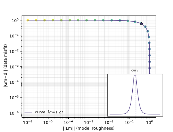
synthetic corner: lambda*=1.27, index 15 of 30

<Axes: xlabel='||Lm|| (model roughness)', ylabel='||Gm−d|| (data misfit)'>
Reading this figure. The classic L shape: a near-vertical branch
at small \(\lambda\) (misfit barely changes, roughness drops
fast) and a near-horizontal branch at large \(\lambda\) (the
opposite) meeting at a corner — marked with a star — which
plot_lcurve() locates automatically. The
small inset shows the underlying curvature score peaking exactly at
that point.
2. A real L-curve from real data#
The rest of this example uses a genuine (if small) Tikhonov smoothing problem: given one station’s real, noisy \(\log_{10}\rho_a(T)\) curve as data \(d\), solve \((I + \lambda^2 D^\top D)\,m = d\) for a smoothed model \(m\), where \(D\) is the second-difference (roughness) operator. Misfit is \(\Vert m-d \Vert\) and roughness is \(\Vert Dm \Vert\) — the same quantities any regularized inversion reports, computed here in closed form.
from _datasets import load_survey  # noqa: E402

from pycsamt.emtools import ensure_sites  # noqa: E402
from pycsamt.emtools._core import (  # noqa: E402
    _get_z_block,
    _iter_items,
    _name,
)

survey = ensure_sites(load_survey("amt_l18plt"), recursive=False)


def _rough_operator(n: int) -> np.ndarray:
    D = np.zeros((n - 2, n))
    for i in range(n - 2):
        D[i, i], D[i, i + 1], D[i, i + 2] = 1.0, -2.0, 1.0
    return D


def tikhonov_sweep(log10_rho: np.ndarray, lambdas: np.ndarray):
    n = log10_rho.size
    D = _rough_operator(n)
    I = np.eye(n)
    misfits, roughs, models = [], [], []
    for lam in lambdas:
        m = np.linalg.solve(I + lam**2 * (D.T @ D), log10_rho)
        misfits.append(np.linalg.norm(m - log10_rho))
        roughs.append(np.linalg.norm(D @ m))
        models.append(m)
    return np.array(misfits), np.array(roughs), np.array(models)


def station_log10_rho(survey, name: str):
    for i, ed in enumerate(_iter_items(survey)):
        if _name(ed, i) == name:
            _, z, fr = _get_z_block(ed)
            rho = 0.2 * np.abs(z[:, 0, 1]) ** 2 / fr
            return np.log10(rho), fr
    raise KeyError(name)


lambdas = np.logspace(-3, 3, 60)
d_18001a, fr_18001a = station_log10_rho(survey, "18-001A")
mi_18001a, ro_18001a, models_18001a = tikhonov_sweep(d_18001a, lambdas)

table = lcurve_table(mi_18001a, ro_18001a, lambdas)
j = table.attrs["corner_idx"]
lam_star = table["lam"].iloc[j]
print(f"18-001A: lambda* = {lam_star:.3g}")

plot_lcurve(mi_18001a, ro_18001a, lambdas, labels=["18-001A"])
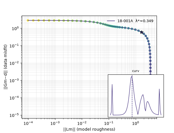
18-001A: lambda* = 0.349

<Axes: xlabel='||Lm|| (model roughness)', ylabel='||Gm−d|| (data misfit)'>
Reading this figure. Real data produces the same qualitative L shape as the synthetic curve in section 1, just noisier — the corner lands at \(\lambda^* \approx 0.35\), comfortably inside the swept range rather than at either end, a first sign that the sweep actually bracketed the useful region.
3. Why the corner matters: three regularization levels#
Plotting the recovered model itself at \(\lambda^*\) against a far smaller (under-regularized) and far larger (over-regularized) choice shows what the corner is actually protecting against.
per_18001a = 1.0 / fr_18001a
j_small = 5  # lambda far below the corner
j_large = 50  # lambda far above the corner

fig, ax = plt.subplots(figsize=(7, 4.5))
ax.semilogx(
    per_18001a, d_18001a, "o", ms=4, color="0.6", label="observed (noisy)"
)
ax.plot(
    per_18001a,
    models_18001a[j_small],
    "-",
    color="#d62728",
    label=f"lambda={lambdas[j_small]:.3g} (under-regularized)",
)
ax.plot(
    per_18001a,
    models_18001a[j],
    "-",
    color="#2ca02c",
    lw=2.2,
    label=f"lambda*={lam_star:.3g} (corner)",
)
ax.plot(
    per_18001a,
    models_18001a[j_large],
    "-",
    color="#1f77b4",
    label=f"lambda={lambdas[j_large]:.3g} (over-regularized)",
)
ax.set_xlabel("Period (s)")
ax.set_ylabel(r"$\log_{10}\rho_a$")
ax.legend(fontsize=7)
ax.set_title("18-001A — effect of the regularization level")
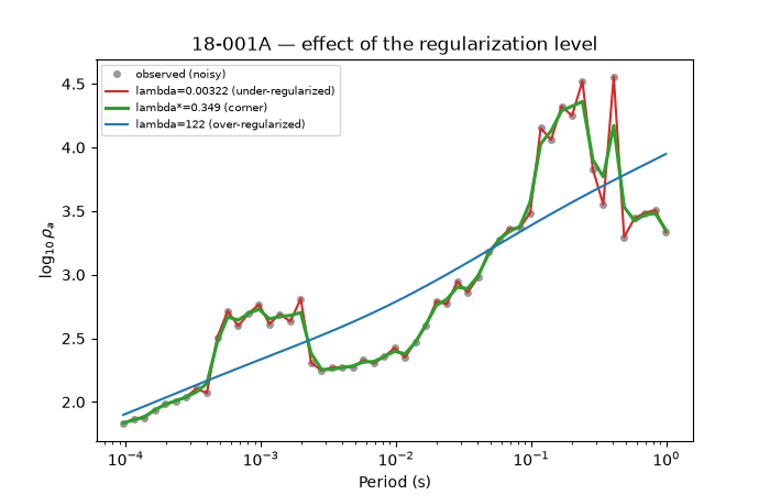
Text(0.5, 1.0, '18-001A — effect of the regularization level')
Reading this figure. The under-regularized model (red) tracks every wiggle in the noisy data — including noise that is almost certainly not real structure. The over-regularized model (blue) is nearly a flat line, discarding real curvature along with the noise. The corner model (green) sits between the two: smoother than the raw data but still following its genuine large-scale shape. This is the practical payoff of the L-curve — picking a defensible middle ground without eyeballing it.
4. Comparing several stations at once#
plot_lcurve() accepts a list of curves
and shares one inset showing every curve’s corner score together.
names = ["18-001A", "18-016A", "18-007U"]
sweeps = {}
for n in names:
    d_n, _ = station_log10_rho(survey, n)
    sweeps[n] = tikhonov_sweep(d_n, lambdas)

plot_lcurve(
    [sweeps[n][0] for n in names],
    [sweeps[n][1] for n in names],
    [lambdas] * len(names),
    labels=names,
)

for n in names:
    t = lcurve_table(sweeps[n][0], sweeps[n][1], lambdas)
    print(f"{n}: lambda* = {t['lam'].iloc[t.attrs['corner_idx']]:.3g}")
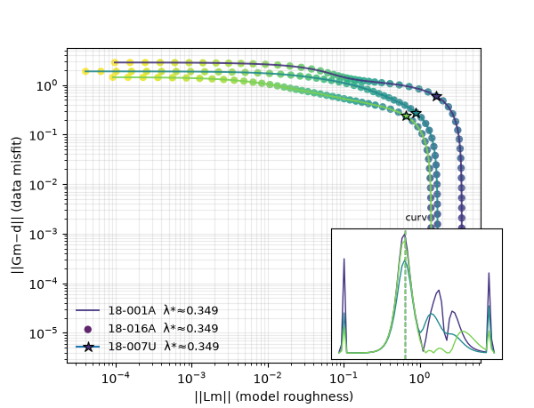
18-001A: lambda* = 0.349
18-016A: lambda* = 0.349
18-007U: lambda* = 0.349
Reading this figure. 18-016A and 18-007U are the same two
stations singled out in the anisotropy/impedance examples for
their unusually strong ratio anisotropy and Swift skew, respectively.
Their L-curves sit at different absolute misfit/roughness levels —
18-001A’s roughness runs highest at every \(\lambda\)
(\(\Vert Lm\Vert\approx 3.57\) at \(\lambda=10^{-3}\)),
18-016A sits in the middle (\(\approx 1.72\)) and
18-007U lowest (\(\approx 1.41\)), consistent with
18-001A being the more structured, less smooth sounding — yet
all three corners land on exactly the same grid index (25 of 60,
\(\lambda^*\approx 0.349\)) despite the very different absolute
resistivity levels behind them. The right relative amount of
smoothing for this survey’s noise character turns out to be
remarkably consistent station to station, even for the two flagged
elsewhere as unusual.
5. Advanced: is the corner pick robust to how it is found?#
method offers "curvature" (numerical second-derivative
curvature of the log-log curve) and "maxdist" (perpendicular
distance from the line joining the curve’s two endpoints), and
smooth controls how much the curve is smoothed before
differentiating for the curvature method specifically.
for sm in (1, 3, 7):
    t_curv = lcurve_table(
        mi_18001a, ro_18001a, lambdas, method="curvature", smooth=sm
    )
    t_dist = lcurve_table(
        mi_18001a, ro_18001a, lambdas, method="maxdist", smooth=sm
    )
    lam_curv = t_curv["lam"].iloc[t_curv.attrs["corner_idx"]]
    lam_dist = t_dist["lam"].iloc[t_dist.attrs["corner_idx"]]
    print(
        f"smooth={sm}: curvature lambda*={lam_curv:.4g}   maxdist lambda*={lam_dist:.4g}"
    )

fig, (axc, axd) = plt.subplots(1, 2, figsize=(11, 4.5), sharey=True)
plot_lcurve(
    mi_18001a, ro_18001a, lambdas, method="curvature", smooth=7, ax=axc
)
axc.set_title("method='curvature', smooth=7")
plot_lcurve(mi_18001a, ro_18001a, lambdas, method="maxdist", smooth=7, ax=axd)
axd.set_title("method='maxdist', smooth=7")
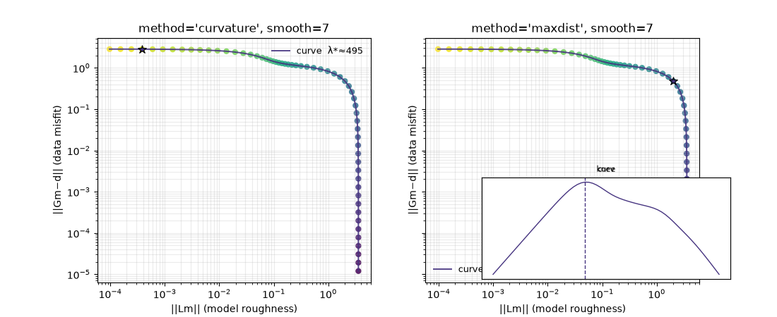
smooth=1: curvature lambda*=0.3486   maxdist lambda*=0.2759
smooth=3: curvature lambda*=0.3486   maxdist lambda*=0.2759
smooth=7: curvature lambda*=495.4   maxdist lambda*=0.2759

Text(0.5, 1.0, "method='maxdist', smooth=7")
Reading this output/figure. At light smoothing (1 or 3), both
methods agree closely (\(\lambda^*\approx 0.35\) vs. 0.28). At
heavy smoothing (smooth=7), the curvature method’s pick jumps to
\(\lambda^*\approx 495\) — essentially the far edge of the sweep,
visibly the wrong corner in the left panel — while maxdist barely
moves, since it never differentiates the curve at all. Heavy
smoothing can silently break the curvature method; maxdist is the
more robust default when in doubt.
6. Advanced: showing the lambda direction along the curve#
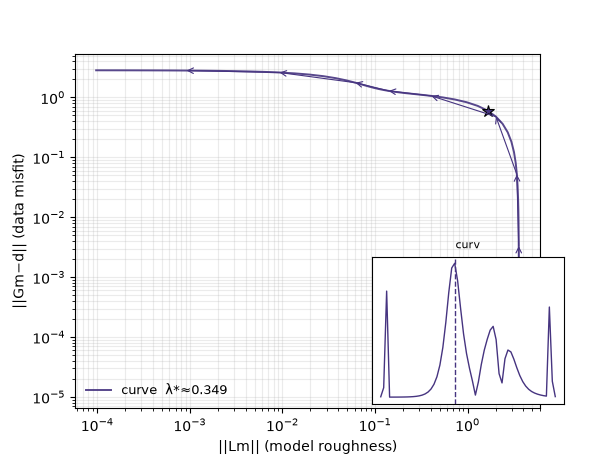
arrow_every draws direction arrows along the path, which is a
useful reminder that a physical parameter sweep — not just point
density — is what “moves” you along an L-curve.
plot_lcurve(mi_18001a, ro_18001a, lambdas, arrow_every=6, show_points=False)
<Axes: xlabel='||Lm|| (model roughness)', ylabel='||Gm−d|| (data misfit)'>
Reading this figure. Arrows point from small to large \(\lambda\). Near the start of the sweep the arrows are almost vertical: roughness barely moves while misfit climbs by orders of magnitude (the model is already close to the data, so a little smoothing costs a lot of fit). Past the corner the arrows turn almost horizontal: roughness keeps falling by decades while misfit grows only slowly — the “cheap” smoothing the corner is meant to capture before this expensive-fit regime takes over. Same two regimes as section 3, now visible directly as a direction of travel along one curve rather than three separate models.
7. Real inversion logs: Occam2D and ModEM#
Sections 1-6 build the L-curve arrays by hand. Real Occam-style
regularized inversion codes already write exactly these three
quantities — misfit, roughness, regularization parameter — to a
convergence log, one row per iteration, because that is what an
Occam-style inversion does at every step. Two adapters read those
logs directly: lcurve_from_occam2d()
and lcurve_from_modem(), each returning
an LCurveData with a .plot() and
.table() shortcut. A third adapter,
lcurve_from_mare2dem(), reads MARE2DEM
logs the same way but is not exercised here — the bundled MARE2DEM
demo run is local-only test data (not checked into the repository),
so an example built on it would not reproduce from a fresh clone.
from _datasets import repo_root  # noqa: E402

from pycsamt.emtools import lcurve_from_modem, lcurve_from_occam2d  # noqa: E402

_DATA = repo_root() / "data"
occam_sweep = lcurve_from_occam2d(_DATA / "occam2D" / "LogFile.logfile")
modem_sweep = lcurve_from_modem(
    _DATA
    / "modem"
    / "willy_27freq_watex_line02_sample"
    / "Modular_NLCG.log"
)
for sweep in (occam_sweep, modem_sweep):
    print(f"{sweep.backend}: {sweep.misfit.size} iterations kept")

fig, axes = plt.subplots(1, 2, figsize=(11, 5))
occam_sweep.plot(
    show_inset=False,
    target_misfit=1.0,
    label_every=4,
    label_prefix="mu=",
    ax=axes[0],
)
axes[0].set_title("Occam2D")
modem_sweep.plot(
    show_inset=False,
    target_misfit=1.05,
    label_every=12,
    label_prefix="lam=",
    ax=axes[1],
)
axes[1].set_title("ModEM")
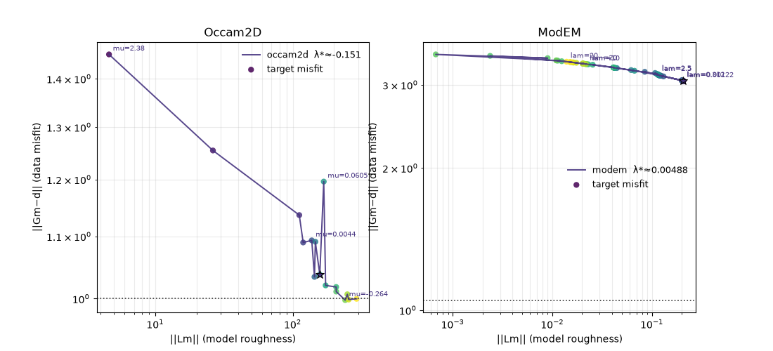
occam2d: 16 iterations kept
modem: 73 iterations kept

Text(0.5, 1.0, 'ModEM')
Reading this figure. Both are real convergence histories, not textbook curves. Occam2D (16 of 17 logged iterations survive — the last stops on “Convergence problems” before writing a roughness) zig zags once it crosses the target RMS, because Occam re-searches its mu whenever a step overshoots. ModEM’s 73-iteration sample never reaches its own configured exit RMS of 1.05 — it is a deliberately compact bundled demo, not a converged production run, and the target line makes that gap honest rather than hiding it inside an axis range that only covers the data.
8. Advanced: do the two corner methods agree on real data?#
Section 5 showed heavy smoothing can break the curvature method on a real but well-behaved curve. Real convergence logs are noisier still, so it is worth checking both methods against each other directly instead of trusting either one blindly.
import pandas as pd  # noqa: E402

rows = []
for name, sweep in (
    ("occam2d", occam_sweep),
    ("modem", modem_sweep),
):
    tc = sweep.table(method="curvature")
    tm = sweep.table(method="maxdist")
    jc, jm = tc.attrs["corner_idx"], tm.attrs["corner_idx"]
    rows.append(
        {
            "backend": name,
            "n_iter": sweep.misfit.size,
            "curv_rough": tc["rough"].iloc[jc],
            "maxdist_rough": tm["rough"].iloc[jm],
        }
    )
print(pd.DataFrame(rows).to_string(index=False))
backend  n_iter  curv_rough  maxdist_rough
occam2d      16  157.348700     168.152600
  modem      73    0.206766       0.000678
Reading this output. Occam2D’s two methods land close together (roughness 157 vs. 168 – both describe the same tight zig-zag near the target). ModEM’s do not: curvature settles on the very last, flattest part of the run (roughness ~0.21) while max-distance picks a point roughly two and a half decades smoother, near the start of the NLCG iteration where the model is still close to its smooth initial guess (roughness ~0.00068) – the real-data version of the smoothing instability from section 5. When the two disagree this much, trust the plotted curve and a known target misfit over either automatic pick.
Total running time of the script: (0 minutes 1.380 seconds)