Plot styles and axis control

Every pycsamt.forward figure is drawn through the library’s shared styling layer, so the same forward result can be re-rendered for different audiences without touching the plotting code. This short example shows the built-in publication and dark styles applied to a 1-D sounding, and how PYCSAMT_CONTROL switches the frequency axis between log-period and linear period.

Note

use_style() and configure_control() set global state. Always pair them with reset_style() (and restore the control) so later figures are unaffected — done here with a try/finally block.

Setup

One sedimentary and one conductive-layer model, each with its MT response, are enough to demonstrate every style.

import matplotlib.pyplot as plt
import numpy as np

from pycsamt.api.control import configure_control
from pycsamt.api.style import reset_style, use_style
from pycsamt.forward import (
    LayeredModel,
    MT1DForward,
    plot_model_1d,
    plot_response_1d,
    plot_response_and_model_1d,
)

# Use the dark-style figure (2nd) as the section thumbnail.

M_SEDIMENTARY = LayeredModel(
    [1_000.0, 20.0, 5.0, 300.0], [200.0, 600.0, 1_500.0], name="sedimentary"
)
M_CONDUCTIVE = LayeredModel(
    [200.0, 5.0, 400.0, 100.0],
    [150.0, 500.0, 2_000.0],
    name="conductive-layer",
)
M_GEOTHERMAL = LayeredModel(
    [500.0, 8.0, 250.0, 3_000.0], [100.0, 400.0, 2_500.0], name="geothermal"
)

FREQS_MT = np.logspace(-3, 4, 35)
R_SED = MT1DForward(FREQS_MT).run(M_SEDIMENTARY)
R_COND = MT1DForward(FREQS_MT).run(M_CONDUCTIVE)
R_GEO = MT1DForward(FREQS_MT).run(M_GEOTHERMAL)

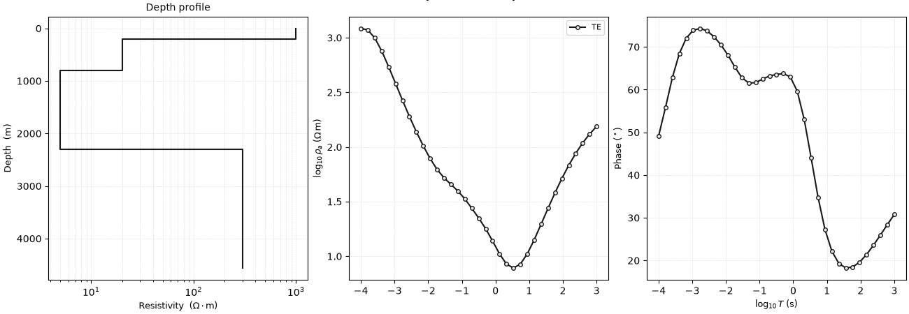
1. Publication style

use_style() swaps in a high-contrast, print-ready palette. We compose the depth profile and the two response panels into a single row using the ax=/axes= arguments.

use_style("publication")
try:
    fig, axs = plt.subplots(1, 3, figsize=(13, 4.5), constrained_layout=True)
    plot_model_1d(M_SEDIMENTARY, ax=axs[0], title="Depth profile")
    plot_response_1d(R_SED, axes=axs[1:3])
    fig.suptitle("Publication style - sedimentary model", y=1.03, fontsize=11)
finally:
    reset_style()

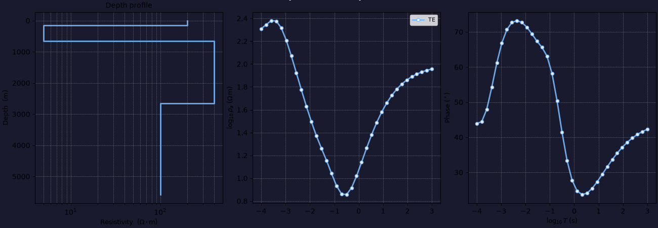
2. Dark style

The dark style targets slides and screens. The figure/axes backgrounds are set explicitly so the whole canvas — not just the plot area — picks up the dark theme.

use_style("dark")
try:
    fig, axs = plt.subplots(
        1, 3, figsize=(13, 4.5), constrained_layout=True, facecolor="#1a1a2e"
    )
    for ax in axs:
        ax.set_facecolor("#1a1a2e")
    plot_model_1d(M_CONDUCTIVE, ax=axs[0], title="Depth profile")
    plot_response_1d(R_COND, axes=axs[1:3])
    fig.suptitle(
        "Dark style - conductive-layer model",
        y=1.03,
        fontsize=11,
        color="white",
    )
finally:
    reset_style()

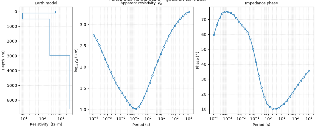
3. Switching the frequency axis

configure_control() changes how every figure maps frequency to the x-axis. Here we switch from the default log10_period to a linear period axis, then restore it so the setting does not leak into other examples.

configure_control(x__view="period")
try:
    fig = plot_response_and_model_1d(
        R_GEO,
        M_GEOTHERMAL,
        title="Period axis (linear scale) - geothermal model",
        figsize=(11, 4.5),
    )
finally:
    configure_control(x__view="log10_period")  # restore default