Comparing network architectures (CNN, ResNet, FCN)

EMInverter1D ships three 1-D architectures — a plain CNN, a residual network (ResNet), and a fully connected network (FCN). Which one to use is an empirical question, so this example trains all three on the same dataset and lays the results out as a comparison grid: convergence curves, a metrics table, prediction residuals, and per-layer error bars.

Shared dataset

One dataset, identical split for every architecture, so differences come only from the networks.

# Use the residual-error grid (3rd figure) as the thumbnail.
import os

import numpy as np

from pycsamt.forward.batch import generate_dataset

# Lighter training while building the docs (PYCSAMT_DOCS_BUILD is set by Sphinx);
# full strength when the example is run directly.
_DOCS = bool(os.environ.get("PYCSAMT_DOCS_BUILD"))

FREQS = np.logspace(-1, 3, 24)
ds = generate_dataset(
    solver="mt1d",
    n_samples=256 if _DOCS else 1200,
    freqs=FREQS,
    n_layers=4,
    noise_level=0.05,
    seed=1,
    verbose=False,
)
train, val, test = ds.split()

Train the three architectures

Each is trained with the same epochs/batch size. We keep the fitted inverter and its training history for the comparisons below.

from pycsamt.ai.inversion.inv1d import EMInverter1D

ARCHS = ["cnn1d", "resnet", "fcn"]
inverters, histories = {}, {}
for arch in ARCHS:
    inv = EMInverter1D(arch=arch, n_layers=4, solver="mt1d")
    inv.fit(train, epochs=6 if _DOCS else 25, batch_size=64, verbose=False)
    inverters[arch] = inv
    histories[arch] = inv._history

Convergence, overlaid

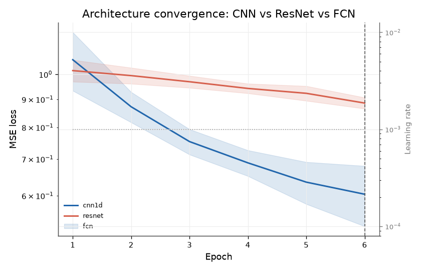
plot_convergence() accepts a list of histories and overlays them, so the learning curves are directly comparable on one axis.

from pycsamt.ai.plot import plot_convergence

fig = plot_convergence(
    [histories[a] for a in ARCHS],
    smoothing=0.2,
    title="Architecture convergence: CNN vs ResNet vs FCN",
)
fig.axes[0].legend(ARCHS, fontsize=8, frameon=False)

<matplotlib.legend.Legend object at 0x7f2aa3943020>

A metrics table

The pycsamt.ai.training metric helpers score each architecture on the held-out test set. We report them on the resistivity parameters (log10 rho, the primary target — all on one scale) rather than mixing in layer thicknesses which live in metres and would dominate the numbers.

from pycsamt.ai import mae, r2, rmse

N_LAYERS = 4
rho = slice(0, N_LAYERS)  # log10-resistivity columns
rows = []
for arch in ARCHS:
    yp = inverters[arch].predict(test.X)
    rows.append(
        (
            arch,
            rmse(test.y[:, rho], yp[:, rho]),
            mae(test.y[:, rho], yp[:, rho]),
            r2(test.y[:, rho], yp[:, rho]),
        )
    )

print(f"{'arch':>8} {'RMSE':>8} {'MAE':>8} {'R^2':>8}   (log10 resistivity)")
for arch, rm, ma, rr in rows:
    print(f"{arch:>8} {rm:8.4f} {ma:8.4f} {rr:8.3f}")

best = min(rows, key=lambda r: r[1])[0]
print("best (lowest resistivity RMSE):", best)

    arch     RMSE      MAE      R^2   (log10 resistivity)
   cnn1d   0.8679   0.7061    0.369
  resnet   0.9655   0.8193    0.219
     fcn   0.9827   0.8211    0.191
best (lowest resistivity RMSE): cnn1d

Residuals of the best model

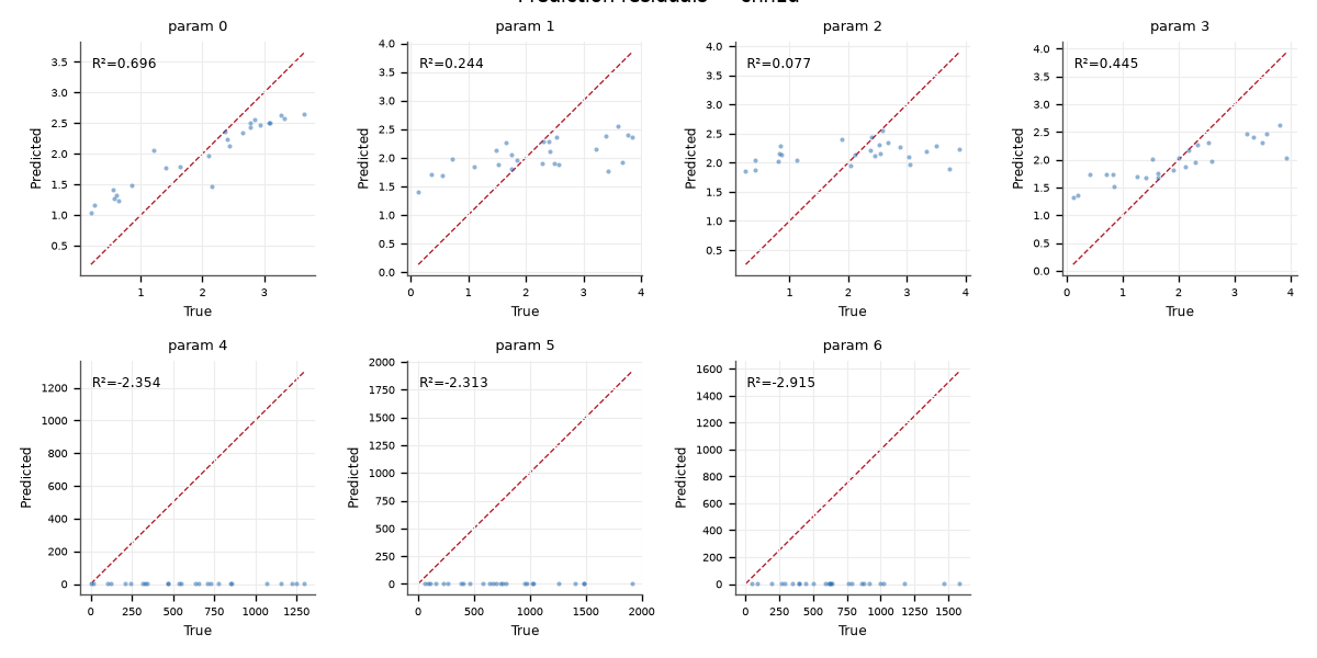
plot_residuals() plots predicted-minus-true per parameter for the best architecture. Tight, unbiased clouds centred on zero mean the network is neither over- nor under-estimating that parameter.

from pycsamt.ai.plot import plot_layer_errors, plot_residuals

y_best = inverters[best].predict(test.X)
fig = plot_residuals(test.y, y_best)
fig.suptitle(f"Prediction residuals — {best}", y=1.02, fontsize=11)

Text(0.5, 1.02, 'Prediction residuals — cnn1d')

Per-layer error

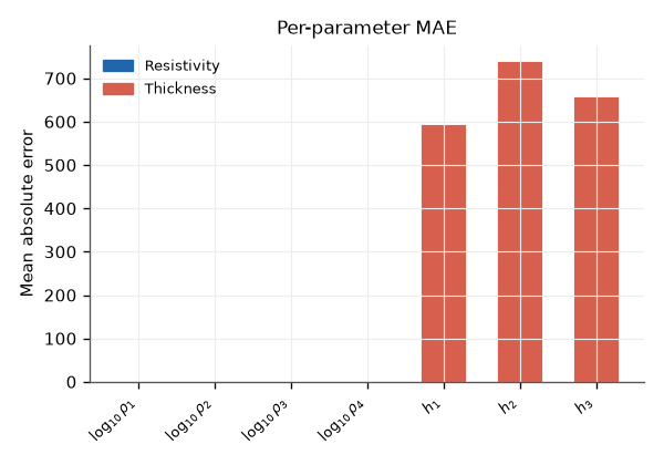
plot_layer_errors() breaks the error down by layer, revealing the classic MT/AMT depth-resolution trade-off: shallow layers are recovered tightly, deeper layers less so.

fig = plot_layer_errors(test.y, y_best, n_layers=4)

Takeaway. On this synthetic task the three architectures land close together, with ResNet and CNN typically edging out the plain FCN. On real data, run exactly this grid on your own training set to pick an architecture — then quantify confidence with Uncertainty and calibration.