Adding a topography strip to a pseudosection

Frequency or period pseudosections do not have a vertical elevation axis, so terrain cannot be draped into the main image the way it can for a depth section. A compact topography strip above the image is the safer display.

This example answers:

How do I show station elevation next to a period/station pseudosection?

We compute apparent resistivity from real WILLY L18PLT impedance data at several frequencies, then add a topography strip with pycsamt.topo.draw_topo_strip().

import os
import sys
from pathlib import Path

import matplotlib.pyplot as plt
import numpy as np


def repo_root():
    root = os.environ.get("PYCSAMT_DOCS_REPO_ROOT")
    return Path(root) if root else Path(__file__).resolve().parents[3]


ROOT = repo_root()
if str(ROOT) not in sys.path:
    sys.path.insert(0, str(ROOT))

from pycsamt.emtools import ensure_sites
from pycsamt.site import SitesReport, res_at_freq
from pycsamt.topo import (
    TopoConfig,
    draw_topo_strip,
    extract_chainage,
    extract_elevation,
    extract_station_names,
)

sites = ensure_sites(
    ROOT / "data" / "AMT" / "WILLY_DATA" / "L18PLT", verbose=0
)
names = extract_station_names(sites)
chain_km = extract_chainage(sites)
elev_m = extract_elevation(sites)
report = SitesReport(sites).to_dataframe(api=False)

1. Build a station-frequency matrix

res_at_freq reports the nearest available frequency per station. The WILLY line has a consistent frequency grid, so this creates a compact pseudosection-like matrix.

freqs = np.array([2.0, 5.0, 10.0, 32.0, 100.0, 320.0, 1000.0, 3200.0])
rho_rows = []
used_rows = []

for freq in freqs:
    df = res_at_freq(sites, float(freq), how="nearest", api=False)
    rho_gmean = np.sqrt(df["res_xy"] * df["res_yx"])
    rho_rows.append(rho_gmean.to_numpy(dtype=float))
    used_rows.append(df["f_used"].to_numpy(dtype=float))

rho_matrix = np.vstack(rho_rows)
used_matrix = np.vstack(used_rows)

print("Requested vs first-station used frequencies:")
for requested, used in zip(freqs, used_matrix[:, 0]):
    print(f"{requested:8.1f} Hz -> {used:8.3f} Hz")

Requested vs first-station used frequencies:
     2.0 Hz ->    2.052 Hz
     5.0 Hz ->    4.990 Hz
    10.0 Hz ->   10.160 Hz
    32.0 Hz ->   29.510 Hz
   100.0 Hz ->  102.400 Hz
   320.0 Hz ->  297.400 Hz
  1000.0 Hz -> 1032.000 Hz
  3200.0 Hz -> 2997.000 Hz

2. Draw a pseudosection with a topography strip

fig, ax = plt.subplots(figsize=(11, 5.6))
image = ax.imshow(
    np.log10(rho_matrix),
    aspect="auto",
    origin="lower",
    cmap="viridis",
    extent=[-0.5, len(names) - 0.5, 0, len(freqs) - 1],
)
ax.set_yticks(np.arange(len(freqs)))
ax.set_yticklabels([f"{f:g}" for f in freqs])
ax.set_xticks(np.arange(len(names))[::3])
ax.set_xticklabels(names[::3], rotation=65, ha="right")
ax.set_xlabel("Station")
ax.set_ylabel("Requested frequency (Hz)")
ax.set_title("L18 apparent-resistivity pseudosection with topography strip")
fig.colorbar(image, ax=ax, label="log10 rho geometric mean")

draw_topo_strip(
    fig,
    ax,
    chain_km,
    elev_m,
    names,
    cfg=TopoConfig(strip_height_ratio=0.18, exaggeration=1.5),
    dark=False,
)

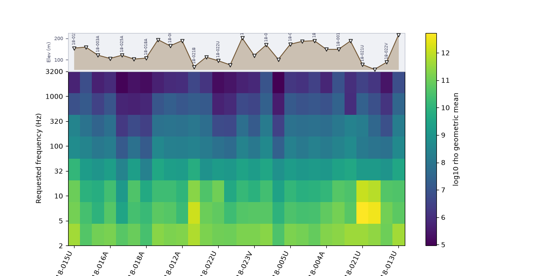
<Axes: ylabel='Elev (m)'>

3. A strip is context, not a depth axis

The topography strip gives the reader station-elevation context, but the pseudosection vertical axis remains frequency. Do not read the strip as a model surface or as terrain-draped depth.

print(
    f"Elevation range shown in strip: {elev_m.min():.1f}-{elev_m.max():.1f} m"
)
print(f"Number of station labels: {len(names)}")

Elevation range shown in strip: 37.0-144.0 m
Number of station labels: 28

Use a strip when the main plot’s y-axis is frequency or period. Use drape_section and draw_topo_section when the main y-axis is actual depth/elevation.