Tipper and induction arrows

The vertical-field transfer function (the tipper) turns into induction arrows that point toward — or away from — lateral conductivity contrasts, a directional constraint the horizontal impedance alone cannot give. The WILLY_DATA AMT lines carry no vertical-field channel, so this final chapter of the survey walkthrough switches to the SAMTEX KAP03 long-period MT line (data/MT/kap03lmt_edis/, 26 stations, periods ~25 s to ~17 ks) — the only bundled survey recorded with a real tipper.

Every figure is from pycsamt.emtools.tf (plus one combined strike-analysis rose from pycsamt.emtools.strike). KAP03 is reproduced here under its SAMTEX attribution; see data/MT/README.md.

Load the tipper-bearing line

KAP03’s measurement axes are geomagnetic-north aligned, so the tipper components sit in a consistent, near-geographic frame. Azimuths below follow each plot’s own north-up, clockwise screen convention.

from _datasets import load_sites

from pycsamt.emtools.strike import plot_strike_analysis
from pycsamt.emtools.tf import (
    plot_induction_arrows,
    plot_induction_convention,
    plot_induction_map,
    plot_induction_rose,
    plot_induction_section,
    plot_tipper_hodograms,
    plot_tipper_polar,
)

KAP = load_sites("mt_kap03")

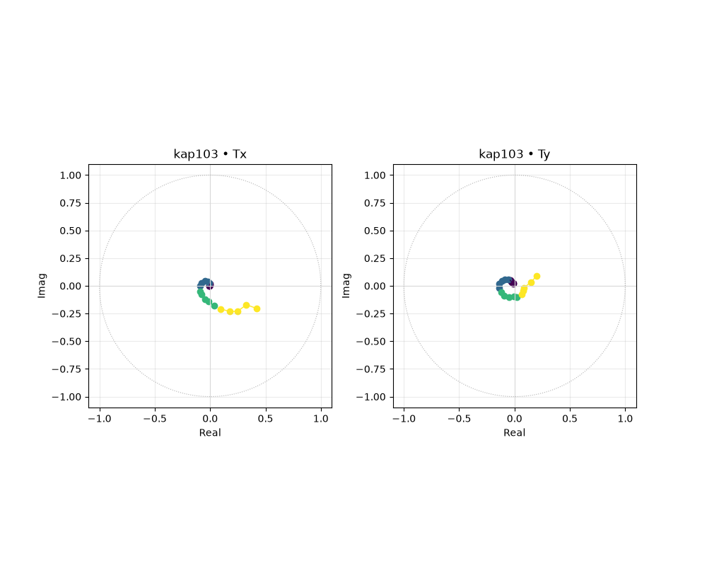
1. Tipper hodograms by period band

plot_tipper_hodograms() traces the real and imaginary tipper vectors on the complex plane, grouped into period bands — the most complete single view of the raw tipper.

plot_tipper_hodograms(KAP, n_bands=4, normalize=False, figsize=(10, 8))

<Figure size 1000x800 with 2 Axes>

2. Tipper polar plots (real and imaginary)

plot_tipper_polar() shows tipper magnitude versus azimuth, one point per frequency, coloured by period. The real part responds to in-phase (nearby) contrasts, the imaginary part to quadrature (deeper or more resistive) ones.

plot_tipper_polar(KAP, component="real", cmap="plasma", figsize=(6, 6))

<PolarAxes: title={'center': 'kap103 — tipper polar [real]'}>

plot_tipper_polar(KAP, component="imag", cmap="viridis", figsize=(6, 6))

<PolarAxes: title={'center': 'kap103 — tipper polar [imag]'}>

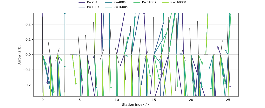
3. Induction arrows across period

plot_induction_arrows() lays out real induction arrows for every station at a set of representative periods spanning KAP03’s band, so you can watch the arrows swing as the sounding depth increases.

plot_induction_arrows(
    KAP,
    periods=[25, 100, 400, 1600, 6400, 16000],
    scale=2.0,
    figsize=(11, 4.5),
)

<Axes: xlabel='Station index / x', ylabel='Arrow (arb.)'>

4. Induction arrow map

plot_induction_map() places the arrows at their station positions for a single period (here 100 s) — the map-view that most directly points at lateral structure.

plot_induction_map(KAP, period=100, scale=0.5, figsize=(7, 5))

<Axes: title={'center': 'Induction arrows  —  T = 100 s  [park]'}, xlabel='x / Easting  (m)', ylabel='y / Northing  (m)'>

5. Tipper magnitude section

plot_induction_section() builds a station-by-period pseudo-section of the (real) tipper magnitude, showing how the vertical-field response is distributed along the line.

plot_induction_section(KAP, component="real", n_periods=20, figsize=(9, 4.5))

<Axes: title={'center': 'Tipper section  [real]'}, xlabel='Station', ylabel='$\\log_{10}(T)$ (s)'>

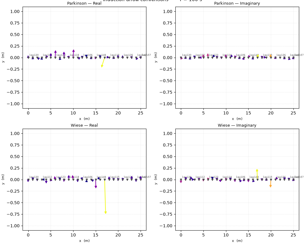
6. Arrow convention reference

plot_induction_convention() is a small reference figure spelling out the sign/direction convention (Parkinson vs Wiese) used by the arrows above, evaluated at 100 s.

plot_induction_convention(KAP, period=100, figsize=(10, 8))

array([[<Axes: title={'center': 'Parkinson — Real'}, xlabel='x  (m)', ylabel='y  (m)'>,
        <Axes: title={'center': 'Parkinson — Imaginary'}, xlabel='x  (m)', ylabel='y  (m)'>],
       [<Axes: title={'center': 'Wiese — Real'}, xlabel='x  (m)', ylabel='y  (m)'>,
        <Axes: title={'center': 'Wiese — Imaginary'}, xlabel='x  (m)', ylabel='y  (m)'>]],
      dtype=object)

7. Induction-arrow azimuth roses (real and imaginary)

plot_induction_rose() folds all arrow azimuths into an axial histogram — the induction-vector counterpart of the strike roses in Geoelectric strike analysis.

plot_induction_rose(KAP, component="real", nbins=36, figsize=(5.5, 5.5))

<PolarAxes: title={'center': 'Induction arrow rose [real]'}>

plot_induction_rose(KAP, component="imag", nbins=36, figsize=(5.5, 5.5))

<PolarAxes: title={'center': 'Induction arrow rose [imag]'}>

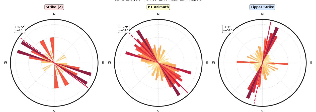
8. Combined strike analysis (Z / phase tensor / tipper)

plot_strike_analysis() puts three independent directional estimates — impedance-tensor strike, phase-tensor azimuth, and tipper strike — in one MTPy-style rose panel, the natural capstone for a tipper-bearing line.

plot_strike_analysis(
    KAP,
    style="pycsamt",
    method="sweep",
    bins=36,
    suptitle="Strike analysis — KAP03  (Z | PT azimuth | Tipper)",
    subplot_size=4.0,
)

<Figure size 1260x450 with 3 Axes>

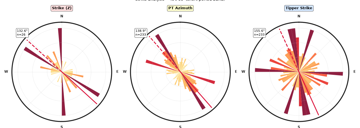
9. Strike analysis, short-period band only

The same three-way comparison restricted to the shortest periods isolates the shallowest structure’s directional signal from the long-period regional trend.

plot_strike_analysis(
    KAP,
    style="pycsamt",
    method="sweep",
    band=(25, 400),
    bins=36,
    suptitle="Strike analysis — KAP03  (short-period band)",
    subplot_size=4.0,
)

<Figure size 1260x450 with 3 Axes>