A publication-ready workflow

The individual waves come together here: static shift, then noise removal, then rotation onto strike, applied in sequence to take the raw survey line to a clean, 2-D-ready dataset. This is the end-to-end recipe you would script for a paper — with a single raw-vs-final comparison to prove the corrections worked.

Chain the corrections

Order matters: remove the vertical static-shift offset first, then clean the curve shape, then rotate onto strike. Each function takes Sites and returns corrected Sites, so the workflow is a simple sequence.

from _corr_data import curves, demo_line, plot_before_after

from pycsamt.emtools import (
    correct_ss_ama,
    rotate_to_strike,
    smooth_rho_phase,
)

raw_sites = demo_line("L18PLT")

step1 = correct_ss_ama(raw_sites, recursive=False)  # static shift
step2 = smooth_rho_phase(
    step1, components="offdiag", robust=True, recursive=False
)  # denoise
final = rotate_to_strike(step2, recursive=False)  # rotate

print(
    "workflow: raw -> static shift -> rho/phi smoothing -> rotate to strike"
)
raw = curves(raw_sites, "rho")
fin = curves(final, "rho")
print(f"{len(raw)} stations processed")

workflow: raw -> static shift -> rho/phi smoothing -> rotate to strike
28 stations processed

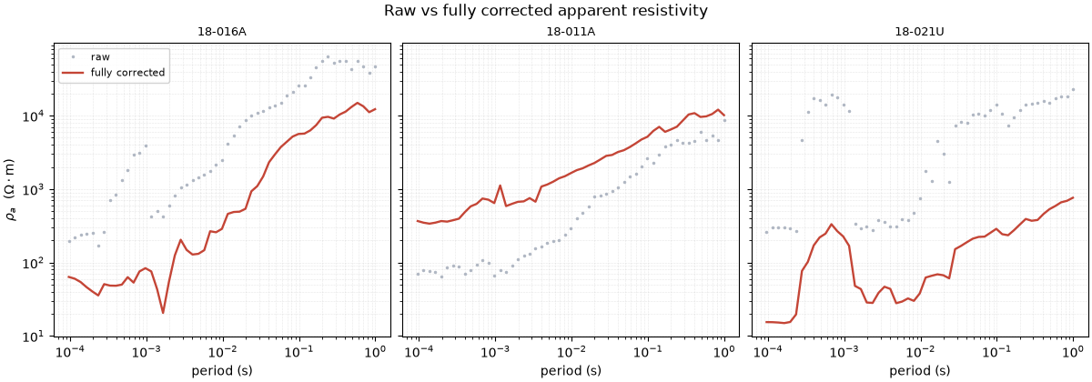
Raw vs fully corrected: apparent resistivity

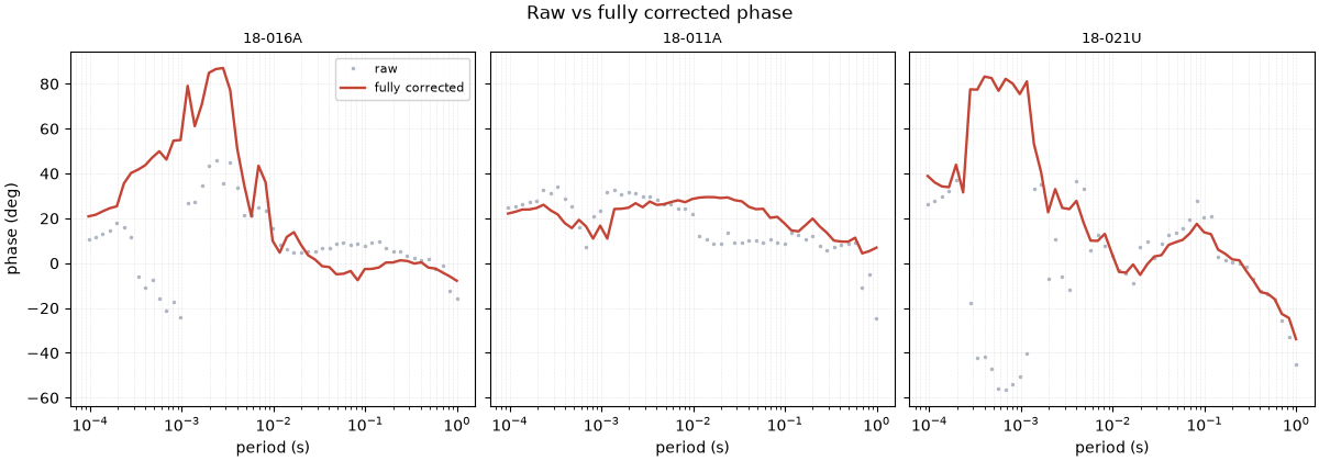
The final curves are collapsed onto a coherent trend (static shift removed), smooth (noise removed), and rotated onto strike — inversion-ready.

stations = list(raw)
pick = [stations[3], stations[len(stations) // 2], stations[-4]]
plot_before_after(
    raw,
    fin,
    pick,
    quantity="rho",
    labels=("raw", "fully corrected"),
    colors=("#b0b7c3", "#c44536"),
    title="Raw vs fully corrected apparent resistivity",
)

<Figure size 1200x420 with 3 Axes>

… and phase

raw_ph = curves(raw_sites, "phase")
fin_ph = curves(final, "phase")
plot_before_after(
    raw_ph,
    fin_ph,
    pick,
    quantity="phase",
    labels=("raw", "fully corrected"),
    colors=("#b0b7c3", "#c44536"),
    title="Raw vs fully corrected phase",
)

<Figure size 1200x420 with 3 Axes>

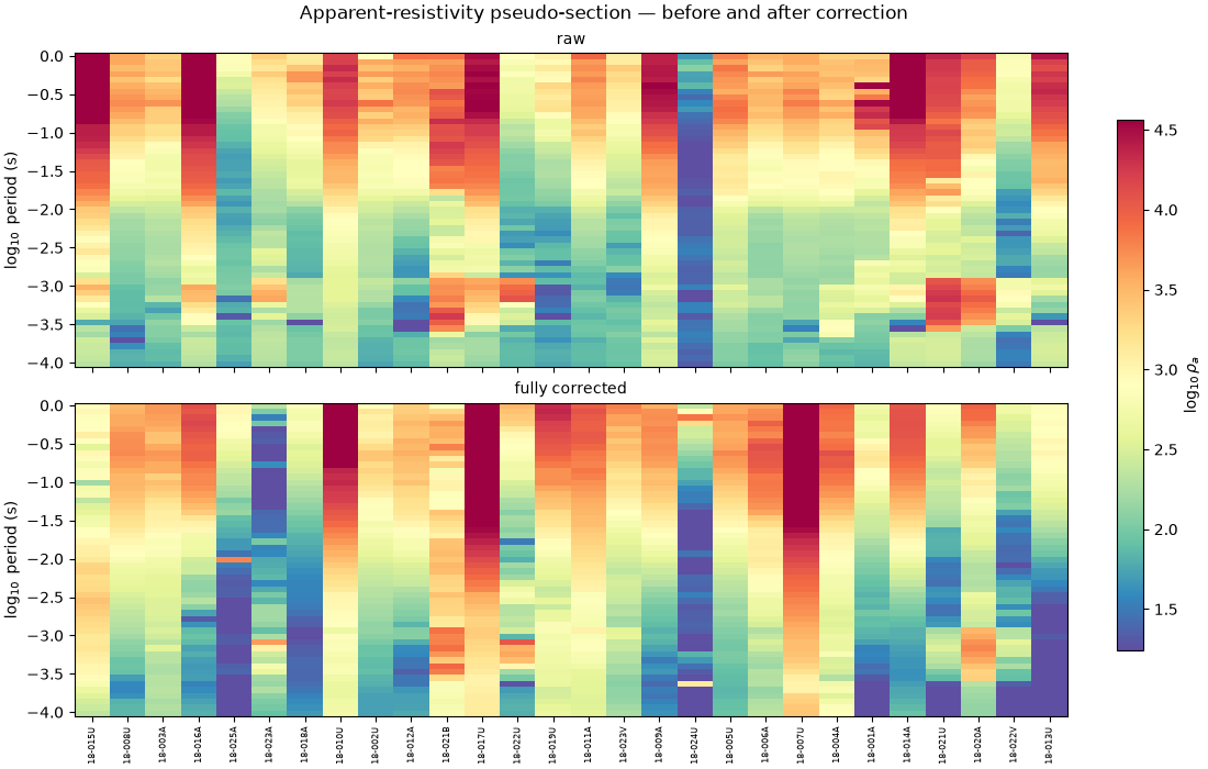
The whole line, before and after

Pseudo-sections of ρ_a across all stations show the corrections at survey scale — the static-shift offsets and curve-to-curve speckle of the raw section are conditioned away and the tensor is re-expressed on strike, leaving a smoother section to hand to the inverter.

import matplotlib.pyplot as plt
import numpy as np

names = [s for s in raw if np.array_equal(raw[s][0], fin[s][0])]
periods = raw[names[0]][0]
R = np.column_stack([np.log10(raw[s][1]) for s in names])
F = np.column_stack([np.log10(fin[s][1]) for s in names])
vmin, vmax = np.nanpercentile(np.concatenate([R, F]), [3, 97])
fig, axes = plt.subplots(
    2, 1, figsize=(11, 7), sharex=True, constrained_layout=True
)
for ax, Z, ttl in [(axes[0], R, "raw"), (axes[1], F, "fully corrected")]:
    im = ax.pcolormesh(
        np.arange(len(names)),
        np.log10(periods),
        Z,
        cmap="Spectral_r",
        vmin=vmin,
        vmax=vmax,
        shading="auto",
    )
    ax.set_ylabel(r"$\log_{10}$ period (s)")
    ax.set_title(ttl, fontsize=10)
axes[1].set_xticks(range(len(names)))
axes[1].set_xticklabels(names, rotation=90, fontsize=6)
fig.colorbar(im, ax=axes, label=r"$\log_{10}\rho_a$", shrink=0.8)
fig.suptitle(
    "Apparent-resistivity pseudo-section — before and after correction",
    fontsize=12,
)

Text(0.5, 0.9940471428571429, 'Apparent-resistivity pseudo-section — before and after correction')

What the corrections did, quantified

Two honest numbers close the workflow. First, how much the data moved — the median \(|\Delta\log_{10}\rho_a|\) per station measures the total conditioning. Second, that the corrections did not degrade the data: build_qc_table()’s median SNR and good-frequency fraction are preserved, so the workflow removed the offset and prepared the geometry without injecting noise or dropping usable frequencies. These steps condition the data — the improvement is structural (the sections above), not a manufactured boost in a single scalar.

from pycsamt.emtools.qc import build_qc_table

moved = np.median(
    [
        np.nanmedian(np.abs(np.log10(fin[s][1]) - np.log10(raw[s][1])))
        for s in names
    ]
)
qc_raw = build_qc_table(raw_sites)
qc_fin = build_qc_table(final)
print(f"median |dlog10 rho_a| moved by the workflow : {moved:.2f}")
print(
    f"median SNR (preserved)                      : "
    f"{qc_raw['snr_med'].mean():.1f} -> {qc_fin['snr_med'].mean():.1f}"
)
print(
    f"good-frequency fraction (preserved)         : "
    f"{qc_raw['frac_ok'].mean():.2f} -> {qc_fin['frac_ok'].mean():.2f}"
)

median |dlog10 rho_a| moved by the workflow : 0.51
median SNR (preserved)                      : 13.4 -> 13.2
good-frequency fraction (preserved)         : 1.00 -> 1.00

Takeaway. Four correction waves — static shift, noise removal, source effects (where relevant), and rotation — turn a raw acquisition into a clean, 2-D-ready dataset, every step a documented pycsamt.emtools call. This is the processing half of the pyCSAMT workflow; the result feeds straight into the classical and AI inverters.